Numerical Treatment and Algorithms

PeleC Time-stepping

PeleC supports two options for time-stepping: a second-order explicit method-of-lines approach (MOL), and an iterative scheme base on a spectral deferred correction approach (SDC). Both time-steppers share a considerable amount of code.

Standard Time Advance

The MOL time stepper is a standard second order predictor-corrector approach with (optional) fixed point iteration to tightly couple the reaction and transport. The advection \((A)\) and diffusion \((D)\) terms are computed using a time-explicit finite-volume formulation; reaction terms are either computed explicitly or integrated (using DVODE or CVODE via SUNDIALS), with a forcing term that incorporates the (pointwise) influence of advection and diffusion (\(F_{AD}\)). The update is as follows:

\[ \begin{align}\begin{aligned}S^n &= AD(u^n) \hspace{2em} {\small \text{(stencils require grow-cell data at }t^{n}\text{)}}\\u^* &= u^n + \Delta t(S^n +I_R)\\S^{n+1} &= AD(u^*) \hspace{2em} {\small \text{(stencils require grow-cell data at }t^{n+1}\text{)}}\\u^{**} &= \frac{1}{2}(u^n+u^*) + \frac{1}{2}\left(S^{n+1}+I_R\right){\Delta t}\\F_{AD} &= \frac{1}{\Delta t} (u^{**} -u^n) - I_R\\I_R &= I_R(u^n, F_{AD})\\u^{n+1} &= u^n + \Delta t(F_{AD} +I_R)\text{.}\end{aligned}\end{align} \]

On initialization, the reaction term \((I_R)\) is evaluated with \((F_{AD} = 0)\); for subsequent time steps, the initial value of \((I_R)\) is taken from the previous time step. The advection and diffusion terms (evaluated above at \(t^n\) and \(t^{n+1}\)) require grow cells to be filled at the appropriate solution time. The filling operation is orchestrated by the AMReX software framework via the FillPatch operation. Grow cells from neighboring mesh patches (and through periodic/re-entrant boundaries) are copied on intersection in index space. User-specified functions provide data at the physical boundaries as a function of space and time. Cells along the coarse-fine boundary are interpolated in space and time from available coarse data (note that this requires that the fine data be “properly nested” in the coarser levels). Also, because \((A)\) and \((D)\) are both time-explicit, they are computed together using grow cells filled by the same FillPatch operation.

With time-implicit reactions, the final update is iterated:

\[ \begin{align}\begin{aligned}S^{n+1,k} &= AD(u^{n+1,k})\\F_{AD}^{k} &= \frac{1}{2}(S^n+S^{n+1,k})\\I_R^{k} &= I_R(u^n, F_{AD}^{k})\\u^{n+1,k+1} &= u^n + \Delta t(F_{AD}^{k} +I_R^{k})\text{.}\end{aligned}\end{align} \]

Hyperbolics

Two hyperbolic treatments are available: Piecewise Parabolic Method and the Method of Lines.

Piecewise Parabolic Method (PPM)

The unsplit piecewise parabolic method is used for regular geometries. Currently in PeleC, there are 2 variants that can be chosen through the ppm_type flag:

• ppm_type = 0 (default) uses a piecewise linear interpolation to reconstruct values at face. This is denoted PLM in the source code.

• ppm_type = 1 is the original PPM method presented in Colella and Woodward [JCP 1984].

For ppm_type = 0, one can control the order of the construction of the slopes with the plm_iorder flag:

• plm_iorder = 1 sets the slopes to zero;

• plm_iorder = 2 uses the \(i-1\), \(i\), and \(i+1\) cells to form a slope;

• plm_iorder = 4 (default) uses the \(i-2\), \(i-1\), \(i\), \(i+1\), and \(i+2\) cells to form a slope.

Note

The following description of PPM implementations are only available in the (deprecated) Fortran source code. Efforts are ongoing to port all the PPM variants into the C++ source code.

Currently in PeleC Fortran source, there are 4 variants that can be chosen through the ppm_type flag:

• ppm_type = 0 uses a piecewise linear interpolation to reconstruct values at face.

• ppm_type = 1 is the original PPM method presented in Colella and Woodward [JCP 1984].

• ppm_type = 2 is the “extrema preserving” variant of the PPM method.

• ppm_type = 3 is a new hybrid PPM/WENO method developed by Motheau and Wakefield [CAMCOS 2020], that replace the interpolation and slope limiting procedures by a WENO reconstruction.

In the remainder of this section, the extrema preserving PPM method, i.e ppm_type = 2, is presented. Note that the implementation in PeleC is a recollection of different extension of the PPM method published in Miller and Colella [JCP 2002] and Colella and Sekora [JCP 2008]. The actual implementation in PeleC is described in the paper Motheau and Wakefield, Investigation of finite-volume methods to capture shocks and turbulence spectra in compressible flows [CAMCOS 2020], and the following description is taken from that paper. Note that the algorithm is presented here in 1D for simplicity, but can be trivially extended to 2D and 3D.

Note also that the hybrid PPM/WENO method is described in the aforementioned paper. This hybrid strategy presents far better results in terms of capture of turbulent spectra rather than the other PPM methods. When ppm_type = 1 and use_hybrid_weno = true is used, the WENO reconstruction method can be selected with weno_scheme:

• weno_scheme = 0 is the classical 5th order WENO-JS of Jiang and Shu [JCP 1996].

• weno_scheme = 1 is the 5th order WENO-Z method of Borges et al. [JCP 2008].

• weno_scheme = 2 is the 7th order WENO-Z.

• weno_scheme = 3 is the 3rd order WENO-Z.

By default, weno_scheme = 1 is selected and use_hybrid_weno = false.

System of primitive variables

First, the system of primitive variables is recast in the following generic form:

\[\frac{\partial \mathbf{Q}}{\partial t} + \mathbf{A} \frac{\partial \mathbf{Q}}{\partial x} = \mathbf{S}_{\mathbf{Q}}. \label{eqn:prim_var_eq}\]

Here \(\mathbf{Q}\) is the primitive state vector, \(\mathbf{A}=\partial \mathbf{F}/\partial \mathbf{Q}\) and \(\mathbf{S}_{\mathbf{Q}}\) are the viscous source terms reformulated in terms of the primitive variables.

In one dimension, this comes:

\[\begin{split}\left(\begin{array}{c} \rho \\ u \\ p \\ \rho e \end{array}\right)_t + \left(\begin{array}{cccc} u & \rho & 0 & 0 \\ 0 & u & \frac{1}{\rho} & 0 \\ 0 & \rho c^2 & u & 0 \\ 0 & \rho e + p & 0 & u \end{array}\right) \left(\begin{array}{c} \rho \\ u \\ p \\ \rho e \end{array}\right)_x = \mathbf{S}_{\mathbf{Q}}\end{split}\]

Note that here, the system of primitive variables has been extended to include an additional equation for the internal energy, denoted \(e\). This avoids several calls to the equation of state, especially in the Riemann solver step.

The eigenvalues of the matrix \(\mathbf{A}_x\) are given by:

\[\mathbf{\Lambda}\left(\mathbf{A}_x\right) = \{u-c,u,u,u+c\}.\]

The right column eigenvectors are:

(1)\[\begin{split}\mathbf{r}_x = \left(\begin{array}{ccccc} 1 & 1 & 0 & 1 \\ -\frac{c}{\rho} & 0 & 0 & \frac{c}{\rho} \\ c^2 & 0 & 0 & c^2 \\ h & 0 & 1 & h \end{array}\right).\end{split}\]

The left row eigenvectors, normalized so that \(\mathbf{l}_x\cdot\mathbf{r}_x = \mathbf{I}\) are:

(2)\[\begin{split}\mathbf{l}_x = \left(\begin{array}{ccccc} 0 & -\frac{\rho}{2c} & \frac{1}{2c^2} & 0 \\ 1 & 0 & -\frac{1}{c^2} & 0 \\ 0 & 0 & -\frac{h}{c^2} & 0 \\ 0 & \frac{\rho}{2c} & \frac{1}{2c^2} & 0 \end{array}\right).\end{split}\]

Note that here, \(c\) and \(h\) are the sound speed and the enthalpy, respectively.

Edge state prediction

The fluxes are reconstructed from time-centered edge state values. Thus, the primitive variables are first interpolated in space with the PPM method, then a characteristic tracing operation is performed to extrapolate in time their values at \(n+1/2\).

• Interpolation and slope limiting

Basically the goal of the algorithm is to compute a left and a right state of the primitive variables at each edge in order to provide inputs for the Riemann problem to solve.

First, the average cross-cell difference is computed for each primitive variable with a quadratic interpolation as follows:

\[\delta q_i = \frac{1}{2} \left(q_{i+1} - q_{i-1}\right).\]

In order to enforce monotonicity, \(\delta q_i\) is limited with the van Leer [1979] method:

\[\delta q_i^* = \min \left(|\delta q_i|,2|q_{i+1}-q_i|,2|q_i - q_{i-1}|\right)\text{sgn}\left(\delta q_i\right),\]

and the interpolation of the primitive values to the cell face \(q_{i+\frac{1}{2}}\) is estimated with:

\[q_{i+\frac{1}{2}} = q_i + \frac{1}{2}\left(q_{i+1}-q_i \right)-\frac{1}{6}\left(\delta q_{i+1}^* - \delta q_i^* \right).\]

In order to enforce that \(q_{i+\frac{1}{2}}\) lies between the adjacent cell averages, the following constraint is imposed:

\[\min\left(q_i,q_{i+1} \right) \leqslant q_{i+\frac{1}{2}} \leqslant \max\left(q_i,q_{i+1} \right).\]

The next step is to set the values of \(q_{R,i-\frac{1}{2}}\) and \(q_{L,i+\frac{1}{2}}\), which are the right and left state at the edges bounding a computational cell. Here, a quartic limiter is employed in order to enforce that the interpolated parabolic profile is monotone. The procedure proposed by Miller [2002] is adopted, which slightly differs from the original one proposed in Colella [1984]. In Miller [2002], this specific procedure is followed by the imposition of another limiter based on a flattening parameter to prevent artificial extrema in the reconstructed values. Here in PeleC, the order of imposition of the different limiting procedures is reversed.

First, the edge state values are defined as:

\[ \begin{align}\begin{aligned}q_{L,i+\frac{1}{2}} = q_{i+\frac{1}{2}},\\q_{R,i-\frac{1}{2}} = q_{i-\frac{1}{2}}.\end{aligned}\end{align} \]

Then the flattening limiter is imposed as follows:

\[ \begin{align}\begin{aligned}q_{L,i+\frac{1}{2}} \leftarrow \chi_i q_{L,i+\frac{1}{2}} + \left(1+\chi_i\right) q_i,\\q_{R,i-\frac{1}{2}} \leftarrow \chi_i q_{R,i-\frac{1}{2}} + \left(1+\chi_i\right) q_i,\end{aligned}\end{align} \]

where \(\chi_i\) is a flattening coefficient computed from the local pressure, and its evaluation is presented below.

A non-dimensional shock resolution parameter \(\beta_{x,ijk}\) is constructed in cell \(ijk\) according to the equation given below.

\[\beta_{x,ijk} = \frac{|P_{i+1,j,k} - P_{i-1,j,k}|}{|P_{i+2,j,k}-P_{i-2,j,k}|}\]

If \(\beta_{x,ijk}\) is small, then any discontinuity is assumed to be well resolved. If \(\beta_{x,ijk}\) is 0.5 then the pressure \(P\) is linear across four consecutive cells in the i-th direction. A minimum value of \(\tilde \chi_{x,i,j,k}\) is now calculated using two additional parameters \(a_0\) and \(a_1\) as,

\[\tilde \chi_{x,i,j,k}^{min} = max(0,min(1,\frac{a_1-\beta}{a_1-a_0}))\]

The values of \(a_0\) and \(a_1\) are fixed as \(0.75\) and \(0.85\) respectively.

The flattening parameter \(\tilde \chi_{x,ijk}\) is now defined as,

\[\begin{split}\tilde \chi_{x,ijk} =\begin{cases} max(\tilde \chi_{x,i,j,k}^{min},min(1,\frac{Z_1-Z_{x,ijk}}{Z_1-Z_0}), & \text{if $q_{x,i+1,j,k}<q_{x,i-1,j,k}$}.\\ 1, & \text{otherwise}. \end{cases}\end{split}\]

with the non-dimensional shock strength parameter \(Z_{x,ijk}\) defined as,

\[Z_{x,ijk} = \frac{|P_{i+1,j,k} - P_{i-1,j,k}|}{\rho c^2}\]

For the case of three-dimensional flows, the limiter \(\chi_{ijk}\) is then computed using the equation given below,

\[\begin{split}\chi_{ijk} = min(\tilde \chi_{x,i-1,j,k},\tilde \chi_{x,i,j,k},\tilde \chi_{x,i+1,j,k},\\ \tilde \chi_{y,i,j-1,k},\tilde \chi_{y,i,j,k},\tilde \chi_{y,i,j+1,k},\tilde \chi_{z,i,j,k-1},\tilde \chi_{z,i,j,k}, \tilde \chi_{z,i,j,k+1}),\end{split}\]

Finally, the monotonization is performed with the following procedure:

\[\begin{split}q_{L,i+\frac{1}{2}} = q_{R,i-\frac{1}{2}} = q_i \hspace{0.8cm} &\text{if} \hspace{0.2cm} \left(q_{L,i+\frac{1}{2}} - q_i \right)\left(q_i - q_{R,i-\frac{1}{2}}\right) > 0, \\ q_{L,i+\frac{1}{2}} = 3 q_i - 2 q_{R,i-\frac{1}{2}} \hspace{0.8cm} &\text{if} \hspace{0.2cm} |q_{L,i+\frac{1}{2}}-q_i| \geqslant 2|q_{R,i-\frac{1}{2}}-q_i|, \\ q_{R,i-\frac{1}{2}} = 3 q_i - 2 q_{L,i+\frac{1}{2}} \hspace{0.8cm} &\text{if} \hspace{0.2cm} |q_{R,i-\frac{1}{2}}-q_i| \geqslant 2|q_{L,i+\frac{1}{2}}-q_i|.\end{split}\]

• Piecewise Parabolic Reconstruction

Once the limited values \(q_{R,i-\frac{1}{2}}\) and \(q_{L,i+\frac{1}{2}}\) are known, the limited piecewise parabolic reconstruction in each cell is done by computing the average value swept out by parabola profile across a face, assuming that it moves at the speed of a characteristic wave \(\lambda_k\). The average is defined by the following integrals:

(3)\[ \begin{align}\begin{aligned} \mathcal{I}^{(k)}_{+} \left(q_i \right) &= \frac{1}{\sigma_k \Delta x}\int^{(i+1/2)\Delta x}_{((i+1/2)-\sigma_k)\Delta x} q_i^I\left(x\right){\rm d}x,\\ \mathcal{I}^{(k)}_{-} \left(q_i \right) &= \frac{1}{\sigma_k \Delta x}\int^{((i-1/2)+\sigma_k)\Delta x}_{(i-1/2)\Delta x} q_i^I\left(x\right){\rm d}x,\end{aligned}\end{align} \]

with \(\sigma_k = |\lambda_k|\Delta t / \Delta x\), where \(\lambda_k=\{u-c,u,u,u+c\}\), while \(\Delta t\) and \(\Delta x\) are the discretization step in time and space, respectively, with the assumption that \(\Delta x\) is constant in the computational domain.

The parabolic profile is defined by

\[q_i^I \left(x\right) = q_{R,i-\frac{1}{2}} + \xi\left(x\right)\left[q_{L,i+\frac{1}{2}} - q_{R,i-\frac{1}{2}} + q_{i,6}\left(1-\xi\left(x\right)\right)\right]\]

with

(4)\[q_{i,6} = 6 q_i - 3\left(q_{R,i-\frac{1}{2}} + q_{L,i+\frac{1}{2}} \right).\]

and

\[\xi \left(x\right) = \frac{x-x_{i-\frac{1}{2}}}{\Delta x}, \hspace{0.8cm} x_{i-\frac{1}{2}} \leqslant x \leqslant x_{i+\frac{1}{2}}\]

Substituting (4) in (3) leads to the following explicit formulations:

\[ \begin{align}\begin{aligned}\mathcal{I}^{(k)}_{+} \left(q_i \right) &= q_{L,i+\frac{1}{2}} - \frac{\sigma_k}{2}\left[q_{L,i+\frac{1}{2}} - q_{L,i+\frac{1}{2}} - \left(1-\frac{2}{3}\sigma_k \right) q_{i,6} \right],\\\mathcal{I}^{(k)}_{-} \left(q_i \right) &= q_{R,i-\frac{1}{2}} + \frac{\sigma_k}{2}\left[q_{L,i+\frac{1}{2}} - q_{L,i+\frac{1}{2}} + \left(1-\frac{2}{3}\sigma_k \right) q_{i,6} \right].\end{aligned}\end{align} \]

• Characteristic tracing and flux reconstruction

The next step is to extrapolate in time the integrals \(\mathcal{I}^{(k)}_{\pm}\) to get the left and right edge states at time \(n+1/2\). This procedure is complex, especially in multi-dimensions where transverse terms are taken into account; the complete detailed procedure can be found in Miller[2002]. In 1D, the left and right edge states are computed as follows:

\[ \begin{align}\begin{aligned}q_{L,i+\frac{1}{2}}^{n+\frac{1}{2}} &= \mathcal{I}^{(k=u+c)}_{+} - \sum_{k:\lambda_k \geqslant 0} \beta_k \mathbf{l}_k \cdot \left[\mathcal{I}^{(k=u+c)}_{+}-\mathcal{I}^{(k)}_{+} \right] \mathbf{r}_k + \frac{\Delta t}{2} S_i^n,\\q_{R,i-\frac{1}{2}}^{n+\frac{1}{2}} &= \mathcal{I}^{(k=u-c)}_{-} - \sum_{k:\lambda_k \leqslant 0} \beta_k \mathbf{l}_k \cdot \left[\mathcal{I}^{(k=u-c)}_{-}-\mathcal{I}^{(k)}_{-} \right] \mathbf{r}_k + \frac{\Delta t}{2} S_i^n.\end{aligned}\end{align} \]

where

\[\begin{split}\beta_k = \begin{cases} \frac{1}{2}, & \text{if}\;\lambda_k = 0, \\ 1, & \text{otherwise}, \end{cases}\end{split}\]

and \(\mathbf{l}_k\) and \(\mathbf{r}_k\) are the left row and right column of the matrices defined at (1) and (2) for each eigenvalue \(k\). Note that here, \(S_i^n\) represents any source terms at time \(n\) to include in the characteristic tracing operation.

Finally, the time-centered fluxes are computed using an approximate Riemann problem solver. At the end of this procedure the primitive variables are centered in time at \(n+1/2\), and in space at the edges of a cell. This is the so-called Godunov state and the convective fluxes can be computed to create the advective source term.

Method of Lines with Characteristic Extrapolation

An alternative formulation well suited to Embedded Boundary geometry treatment and also available for regular grids is available and based on a method of lines approach. For each direction, characteristic extrapolation is used to compute left and right states at the cell faces:

\[ \begin{align}\begin{aligned}{u^l_\perp} = u^- + \frac{1}{2\rho^-}\left( \alpha^-_2 - \alpha^-_1\right)\\{p^l} = p^- + \frac{c}{2}\left( \alpha^-_2 +\alpha^-_1\right)\\u^l_{\parallel, 1} = v^- + \frac{1}{2} \alpha^-_3\\u^l_{\parallel, 2} = w^- + \frac{1}{2} \alpha^-_4\\\rho^l Y_k^l = Y_k^-\rho^- + \frac{1}{2c}\left[\alpha^-_{4+k} + Y_k^-\left(\alpha^-_1 + \alpha^-_2\right)\right]\\\rho^l = \sum{\rho^lY_k^l}\\Y_k^l = \frac{\rho^l Y_k^l}{\rho^l}\end{aligned}\end{align} \]

The right states are computed as:

\[ \begin{align}\begin{aligned}{u^r_\perp} = u^+ - \frac{1}{2\rho^+}\left( \alpha^+_2 - \alpha^+_1\right)\\{p^r} = p^+ - \frac{c}{2}\left( \alpha^+_2 +\alpha^+_1\right)\\u^r_{\parallel, 1} = v^- - \frac{1}{2} \alpha^-_3\\u^r_{\parallel, 2} = w^- - \frac{1}{2} \alpha^-_4\\\rho^r Y_k^r = Y_k^+\rho^+ - \frac{1}{2c}\left[\alpha^+_{4+k} + Y_k^+\left(\alpha^+_1 + \alpha^+_2\right)\right]\\\rho^r = \sum{\rho^rY_k^r}\\Y_k^r = \frac{\rho^r Y_k^r}{\rho^r}\end{aligned}\end{align} \]

The computations in the y- and z- direction are analogous; the flux on an EB face to apply a no-slip boundary condition at a wall is somewhat different. In that case, the left and right states are taken as the state at the cell center, except for the velocity is reflected across the EB face. That is:

\[ \begin{align}\begin{aligned}u^l_\perp = - u \cdot \vec{n}\\u^l_{\parallel, 1} = u^l_{\parallel_2} = 0.0\\p^l = p\\Y_k^l = Y_k\\\rho^l = \rho\end{aligned}\end{align} \]

and, as noted the right state is identical except for:

\[u^r_\perp = - u^l_\perp\]

Once the left and right states are computed, a Riemann solver (in this case one preserving the physical constraints on the intermediate state) is used to compute fluxes that are assembled into a conservative and non-conservative update for the regular and cut cells.

The characteristic extrapolation requires (slope limited) fluxes, which computes the slope routines compute (limited) slopes as:

\[ \begin{align}\begin{aligned}\Delta_1^- = 0.5\frac{1}{c}\left(p-p^-\right) - 0.5 \rho \left( u - u^-\right)\\\Delta_2^- = 0.5\frac{1}{c}\left(p-p^-\right) + 0.5 \rho \left( u - u^-\right)\\\Delta_3^- = v - v^-\\\Delta_4^- = w - w^-\\\Delta^-_{k=5..nspecies} = \rho Y_k - \rho^- Y_k^- - \frac{1}{c^2}Y_k \left(p-p^-\right)\end{aligned}\end{align} \]

If cell is irregular, or neighbor to left is irregular, \(\Delta^- = 0.0\).

\[ \begin{align}\begin{aligned}\Delta_1^+ = 0.5\frac{1}{c}\left(p^+ - p\right) - 0.5\rho\left(u^+ - u\right)\\\Delta_2^+ = 0.5\frac{1}{c}\left(p^+ - p\right) + 0.5\rho\left(u^+ - u\right)\\\Delta_3^+ = v^+ - v\\\Delta_4^+ = w^+ - w\\\Delta_{5...nspc}^+ = \rho^+ Y_k^+ - \rho Y_k - \frac{Y_k}{c^2}\left(p^+ - p \right)\end{aligned}\end{align} \]

Again, if cell is irregular, or neighbor to right is irregular, \(\Delta^+ = 0.0\). Finally, the slopes are limited according to:

\[ \begin{align}\begin{aligned}\Delta_i = \frac{1}{2}\left(\Delta_i^- + \Delta_i^+\right)\\\alpha_i^{\mathrm{lim}} = \mathrm{sign}\left\{\Delta_i \right\} \cdot \min\left\{ \Delta^{lim}_i, \left|\Delta_i \right|\right\}\end{aligned}\end{align} \]

where:

\[\begin{split}\Delta^{lim} = \left\{ \begin{aligned} {} 2 \min\left\{ |\Delta^-|,|\Delta^+|\right\} \quad& \mathrm{if} \Delta^- \cdot \Delta^+ \ge 0 \\ 0 & \quad \mathrm{otherwise}\end{aligned}\right.\end{split}\]

The formulation of the y- and z-directions is analogous to the x-direction. One can control the order of the construction of the slopes with the mol_iorder flag:

• mol_iorder = 1 sets the slopes to zero;

• mol_iorder = 2 uses the procedure described above.

Comparison of PPM and MOL for the decay of homogeneous isotropic turbulence

Comparison of PPM and MOL were performed using the decay of homogeneous isotropic turbulence. Initial conditions for the velocity fields were provided by an incompressible spectral simulation. The comparisons were performed at \(N=128^3\) and \(512^3\). While generally exhibiting similar results, the MOL is more dissipative that the PPM, as shown in the figure below. For the MOL at \(N = 512^3\), the maximum relative error in kinetic energy is \(0.9\%\) and \(k_{90}= 3 k_{\lambda_0}\) at \(t=5\tau\), for the PPM, these numbers are \(0.5\%\) and \(4 k_{\lambda_0}\). The dissipation rate is under-predicted for the MOL. The energy spectra at high wave-numbers for the MOL are lower than those for the PPM. Finally, the MOL has a more restrictive CFL condition (CFL=0.3), and, therefore, MOL simulations were approximately three times slower than PPM simulations.

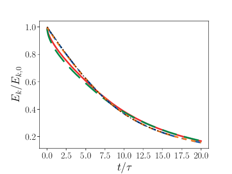
1 Kinetic energy as a function of time. Solid red: PPM at \(N=128^3\); dashed green: MOL at \(N=128^3\); dot-dashed blue: PPM at \(N=512^3\); dotted orange: MOL at \(N=512^3\); dashed black: spectral code.

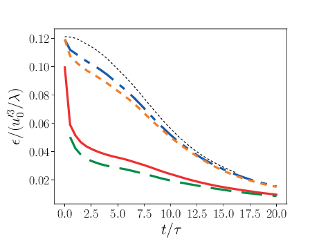
2 Dissipation as a function of time. Solid red: PPM at \(N=128^3\); dashed green: MOL at \(N=128^3\); dot-dashed blue: PPM at \(N=512^3\); dotted orange: MOL at \(N=512^3\); dashed black: spectral code.

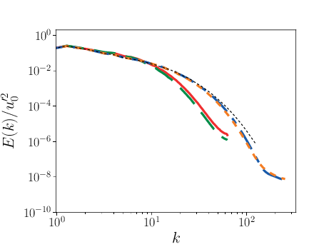
3 Three dimensional energy spectrum at \(t = 5\tau\). Solid red: PPM at \(N=128^3\); dashed green: MOL at \(N=128^3\); dot-dashed blue: PPM at \(N=512^3\); dotted orange: MOL at \(N=512^3\); dashed black: spectral code.

Advection schemes and EB

The two main advection schemes (PLM and MOL) described above support the use of complex geometry in the domain (as implemented using the Embedded Boundary (EB) formulation). While the PLM advection scheme is preferred numerically (less dissipative scheme), the PLM implementation with EB is a recent addition and has not had the same extensive testing as the MOL scheme with EB. Both PLM and MOL may also have issues when the EB intersects the boundary at an angle (this remains to be solved).

Diffusion

One of two diffusion models is selected during the compilation of PeleC, based on the choice of the equation-of-state: a simple model for ideal gases, and a more involved model when real gases are employed. In both cases, the associated derivatives are discretized in space with a straightforward centered finite-volume approach. Transport coefficients (discussed below) are computed at cell centers from the evolving state data, and are arithmetically averaged to cell faces where they are needed to evaluate the transport fluxes. The time discretization for the transport terms is fully explicit and second-order. Although formally this approach leads to a maximum \(\Delta t\) restriction for time evolution that scales as \(\Delta x^2\), it is well known that for resolved flows the CFL constraint will provide the most restrictive time step limitation (ignoring chemical times). Note that when subgrid models are employed for advection, or stiff reactions are incorporated with an explicit treatment of chemistry, the maximum achievable \(\Delta t\) may be considerably smaller than the CFL limit, and other integration approaches might perform significantly better.

Ideal Gas Diffusion

To close the system for a mixture of ideal gases, we adopt the definition for internal energy used in the CHEMKIN standard,

\[e=\sum_m Y_m e_m(T)\]

where \(e_m\) is the species \(m\) internal energy, as specified in the thermodynamics database for the mixture. For ideal gases, the transport fluxes can be written as:

\[ \begin{align}\begin{aligned}&&\boldsymbol{\mathcal{F}}_{m} = \rho Y_m \boldsymbol{V_m} = - \rho D_{m,mix} \nabla X_m\\&&\Pi_{i,j} = \frac{2}{3} \mu \delta_{i,j} \frac{\partial {u_k}}{\partial x_k} - \mu \Big( \frac{\partial u_i}{\partial x_j} + \frac{\partial u_j}{\partial x_i}\Big)\\&&\boldsymbol{\mathcal{Q}} = \sum_m h_m \boldsymbol{\mathcal{F}}_{m} - \lambda \nabla T\end{aligned}\end{align} \]

The mixture-averaged transport coefficients discussed above (\(\mu\), \(\lambda\) and \(D_{m,mix}\)) can be evaluated from transport properties of the pure species. We follow the treatment used in the EGLib library, based on the theory/approximations developed by Ern and Givangigli (however, PeleC uses a recoded version of these routines that are thread safe and vectorize well on suitable processors).

The following choices are currently implemented in PeleC

• The viscosity, \(\mu\), is estimated based on an empirical mixture formula (with \(\alpha = 6\)):

\[\mu = \Big( \sum_m X_m (\mu_m)^{\alpha} \Big)^{1/\alpha}\]

• The conductivity, \(\lambda\), is also calculated using a similar formula as that \(\mu\) but with \(\alpha = 1/4\):

\[\lambda = \Big( \sum_m X_m (\lambda_m)^{\alpha} \Big)^{1/\alpha}\]

• The diffusion flux is approximated using the diagonal matrix \(diag(\widetilde{ \Upsilon})\), where:

\[\widetilde{ \Upsilon}_m = D_{m,mix}, \;\;\;\mbox{where} \;\;\; D_{m,mix} = \frac{1-Y_m}{ \sum_{j \neq m} X_j / \mathcal{D}_{m,j}}\]

This leads to a mixture-averaged approximation that is similar to that of Hirschfelder-Curtiss:

\[\rho Y_m \boldsymbol{V_m} = - \rho D_{m,mix} \nabla X_m\]

Note that with these definitions, there is no guarantee that \(\sum \boldsymbol{\mathcal{F}}_{m} = 0\), as required for mass conservation. An arbitrary correction flux, consistent with the mixture-averaged diffusion approximation, is added in PeleC to enforce conservation.

The pure species and mixture transport properties are evaluated with (thread-safe, vectorized) EGLib functions, which require as input polynomial fits of the logarithm of each quantity versus the logarithm of the temperature.

\[ln(q_m) = \sum_{n=1}^4 a_{q,m,n} ln(T)^{(n-1)}\]

\(q_m\) represents \(\eta_m\), \(\lambda_m\) or \(D_{m,j}\). These fits are generated as part of a preprocessing step managed by the tool FUEGO based on the formula (and input data) discussed above. The role of FUEGO to preprocess the model parameters for transport as well as chemical kinetics and thermodynamics, is discussed in some detail in <Section FuegoDescr>.

Reaction

A chemical reaction network is evaluated to determine the reaction source term. The reaction network is selected at build time by setting the CHEMISTRY_MODEL flag in the makefile, where the value refers to one of the models available in PelePhysics. New models can be generated using Fuego, currently not part of PelePhysics but slated for inclusion in the near future.

Equation of State

Several equation of state models are available based on ideal gas, gamma law gas or non-ideal equation of state. These are implemented through the PelePhysics module.