Geometry treatment in PeleC
The treatment of geometric features that do not align along cartesian coordinate directions effectively reduces to determining the correct flux terms at cut-cell interfaces and subsequent update of divergence term in each cell. This involves the initialization and query of the necessary AMReX-provided data structures containing the geometry information, and computation of PeleC-specific advection and diffusion operators. The various steps in the process are:
Creation of a functional specification of the irregular geometry to embed in the uniform grid. This is done via exact function representations of the geometry or implicit functions.
Construction of map of the (continuous) implicit representation of geometry onto the discrete mesh on all AMR levels. This will be a large, complex, distributed data structure.
Communication of the subsets of this large data set to the local cores tasked with building the PeleC operators.
Actual construction of the diffusion and advection components of the PeleC time advance.
AMReX data structures and functions provide for the first 3 steps. Step 4 is implemented using a “method-of-lines” update within PeleC (see section MOL).
Embedded Boundary Representation
4 Embedded boundary representation of geometry
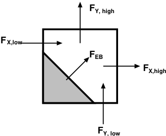
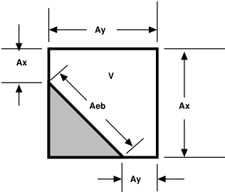
Geometry is treated in PeleC using an embedded boundary (EB) formulation, based on datastructures and algorithmic components provided by AMReX. In the EB formalism, geometry is represented by volume fractions (\(v_l\)) and apertures (\(A_l^k\)) for each cell \(l\) that have faces \(1,...,k,6\). See Embedded boundary representation of geometry for an illustration where the grey area represents the region excluded from the solution domain and the arrows represent fluxes. The fluid volume in a given cell is given by (\(V_l = v_l\,\,dx\,dy\,dz`=v_l\,dx^3\)); it should be noted that the grid spacing along each direction is the same in PeleC.
5 Embedded boundary representation of geometry
6 Embedded boundary representation of geometry
The geometry components in AMReX are used in PeleC to implement a time-explicit integrator based on the method-of-lines. For the advection and diffusion components of the PeleC time integrator, the time rate of change of the conserved fields, S, in cell \(l\) can be written as
where \(F\) is the intensive flux of \(S\) through the faces that bound the cell.
Redistribution
A straightforward implementation of the finite-volume advance of intensive conserved fields is numerically unstable (this is the well-known “small cell issue”) due to presence of the fluid cell volume in the denominator of the conservative divergence (\((DC)_l\)):
where \(k_l\) is the number of regular and cut faces surrounding cell \(l\) and \(F_k\) is the intensive flux at the centroid of face \(k\).
There are a number of ways to deal with this “small cell issue” and the reader is referred to the relevant discussion in Berger, Marsha, and Andrew Giuliani. “A state redistribution algorithm for finite volume schemes on cut cell meshes.” Journal of Computational Physics 428 (2021): 109820 and Giuliani, Andrew et al. “A weighted state redistribution algorithm for embedded boundary grids” Journal of Computational Physics 464 (2022): 111305. PeleC supports the different types of redistributions described in the papers and implemented in AMReX, using the keyword pelec.redistribution_type, which can have the following values:
"NoRedist": no redistribution"FluxRedist": flux redistribution"StateRedist": weighted state redistribution
The “StateRedist” approach is the default and recommended approach. Part of this algorithm involves using limited, least squares slopes to reconstruct the state within merged cells. The slopes for each state variable are limited individually, which may introduce inconsistency between the internal energy and density that leads to negative temperatures. Therefore, these slopes are set to zero by default in PeleC for robustness. Advanced users wishing to use this feature to maintain 2nd order accuracy at the EB surface may do so by setting pelec.eb_srd_max_order = 2 in their input file.
Mass fractions at the EB
At the EB, it is possible for the hydrodynamics and diffusion operators to create out-of-bounds mass fractions (\(< 0\) or \(>1\)). This can happen for a variety of reasons, including because of the redistribution scheme and the flux interpolation. If this happens, a clipping procedure is applied. This clipping happens after the redistribution scheme. The divergence is used to compute an updated state. A clipping and renormalization is applied to this updated state in cells that (1) have out-of-bounds mass fractions, and (2) are a cut cell or contain a cut cell within neighborhood of one (these are affected by the redistribution scheme). The species are clipped to \(0 \geq \rho Y \geq \rho\). A new density is computed from these clipped values. The kinetic energy is preserved and the internal energy, total energy, and momentum is adjusted with the new density. This updated state is then used to compute an updated divergence (by differencing with the original state).
This can be controlled in the code with:
"eb_clean_massfrac": flag to activate clipping (default to true)"eb_clean_massfrac_threshold": threshold for clipping, clipping is turned on if \(Y < -\epsilon\) or \(1+\epsilon < Y\) (default to 0)
Re-redistribution
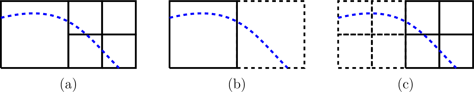
7 (a) an example situation with an EB spanning a coarse-fine boundary, (b) same situation as seen by the coarse level and (c) same situation as seen by the fine level. The cells with the dotted lines are ghost cells.
The redistribution of mass with the use of hybrid divergence method leads to an accounting problem at coarse-fine interfaces that have an EB passing through them, as shown in re-redistribution figure (a). The correct strategy will be to redistribute mass from the coarse mesh on the left side to the fine mesh on the right and vice-versa, when divergence is evaluated on the fly. This strategy is difficult to implement directly into the current algorithmic framework, because flux/residual calculation and time advance are done separately at each level with a ghost-cell treatment at coarse-fine boundaries. Therefore the mass distributed to and from ghost-cells need to be accounted and adjusted after each level has advanced a single time step, which we refer to as re-redistribution. Specifically, four different mass terms need to be accounted for:
In re-redistribution figure (b) the left-coarse-real-cell distributes mass to the right-coarse-ghost-cell. This needs to be captured and given to the right-fine-real-cells.
In re-redistribution figure (b) the right-coarse-ghost-cell distributes mass to the left-coarse-real-cell. This needs to be captured and removed from the left-coarse-real-cell update because the correct distributed mass has to come from the right-fine-real-cells.
In re-redistribution figure (c) the right-fine-real-cells distribute mass to the left-fine-ghost-cells. This needs to be captured and given to the left-coarse-real-cell.
In re-redistribution figure (c) the left-fine-ghost-cells distribute mass to the right-fine-real-cells. This needs to be captured and removed from the right-fine-real-cells update because the correct distributed mass has to come from the left-coarse-real-cell.
The re-redistribution is implemented as a book-keeping step where the mass distributed are stored during MOL divergence calculation and given to the coarse and fine flux registers to reflux at the end of each time step. The re-redistribution is performed every time the reflux function is called in post_timestep. More details regarding re-redistribution are presented in Pember et al.. A forthcoming paper will describe the methodology for this procedure when using state redistribution.
Data Structures and utility functions
Several structures exist to store geometry dependent information. These are populated on creation of a new AMRLevel and stored in the PeleC object so that they are available for computation. These facilitate accessing the EB data. The datatypes are:
C++ struct |
Contents |
|---|---|
EBBoundaryGeom |
Cut face normal, centroid, area, index into FAB |
EBBndrySten |
\(3^3\) matrix of weights to apply cell based stencil, BC value, index into FAB |
FaceSten |
\(3^2\) matrix of weights to apply face-based stencil |
An array of structures is created on level creation by copying data from the AMReX dense datastructures on a per-FAB basis as indicated in Figure Storage for sparse EB structures .
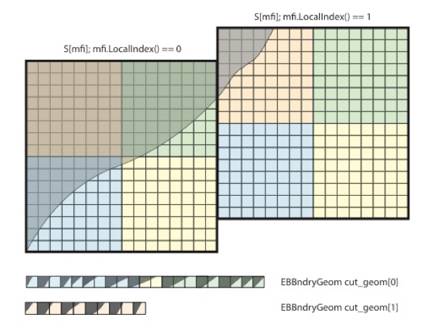
8 Storage for sparse EB structures
On creation of a new AMRLevel, data is cached from the dense AMReX structures in the sparse PeleC structures.
Applying boundary and face stencils
When processing geometry cells, the cached datastructures can be applied efficiently, for example, to interpolate fluxes from face centers to face centroids in cut cells. Two stencil types are available for computing the gradients at the EB for diffusive fluxes, and they are selected as follows:
ebd.boundary_grad_stencil_type = 0: Quadratic stencil (default). On poorly resolved geometries, this stencil may reach into covered cells, in which case the simulation will fail with a warning. See Johansen and Collela for further details.ebd.boundary_grad_stencil_type = 1: Least-squares stencil. See Anderson and Bonhaus for further details.
Geometry initialization
Creating an EB geometry also requires knowledge of the finest level that will be used so that geometries that ‘telescope’, i.e., coarser volume fractions are consistent with applying the coarsening operator to the finer volumes, can be created. To that end there is a global geometry creation step, facilitated by the initialize_EB2 function, as well as a step that happens when a new AMRLevel is created. The latter happens by a call to PeleC::initialize_eb2_structs through PeleC::init_eb called from the PeleC constructor. Following construction of the geometry, the geometric information is copied into the structures described in the previous section and the various interpolation stencils are populated.
Cartesian grid, embedded boundary (EB) methods are methods where the geometric description is formed by cutting a Cartesian mesh with surface of the geometry. AMReX’s methods to handle EB geometry information, and PeleC’s treatment of the EB aware update could use many possible sources for geometric description. The necessary information is, on a per-cell basis:
Apertures for faces intersected by cut cells,
cut cell volumes that ‘telescope’, that is, volumes at a coarser level are consistent with averaging the volumes from finer levels,
connectivity indicating which neighbor cells are connected to a given cell, and
coordinates of cell and face centroids.
Additionally, the algorithms ultimately require surface normals, but these can be trivially recomputed from the aperture.
GeometryShop and Implicit Functions
One of the greatest advantages of EB technology is that grid generation is robust and fast and can be done to any accuracy as described by Schwartz et al. The foundation class that AMReX uses for geometry generation is called GeometryShop. This class is used to initialize geometric information and associated connectivity graph stored in a distributed database class EBIndexSpace. Historically, the EBIndexSpace database was developed to be used throughout a calculation. Here, we use it only to populate datastructures that can be accessed efficiently in the patterns representative of the Pele motivating problem space.
Given an implicit function \(I\),
GeometryShopinterprets the surface upon which \(I(\mathbf{x}) = 0\) as the surface with which to cut the grid cells.GeometryShopinterprets the positive regions of the implicit function (\(\mathbf{x}: I(\mathbf{x}) > 0\)) as covered by the geometry and negative regions (\(\mathbf{x}: I(\mathbf{x}) < 0\)) as part of the solution domain. For example, if one defines her implicit function \(S\) as
the solution domain would be the interior of a sphere of radius \(R\). Reverse the sign of \(S\) and the solution domain would be the exterior of the sphere. More details are available here.
Specifying basic geometries in input files
There are several basic geometries that are available in AMReX that can be easily specified in the input file, some of which are shown below:
Plane - needs a point (plane_point) and normal (plane_normal).
Sphere - needs center (sphere_center), radius (sphere_radius) and fluid inside/outside flag (sphere_has_fluid_inside).
Cylinder - needs center (cylinder_center), radius (cylinder_radius), height (cylinder_height), direction (cylinder_direction) and fluid inside/outside flag (cylinder_has_fluid_inside).
Box - needs the lower corner (box_lo), upper corner (box_hi) and fluid inside/outside flag (box_has_fluid_inside). The box is aligned along coordinate directions.
Spline - needs a vector of points to create a 2D function that is a combination of spline and line elements. Currently, this geometry does not have a user interface from the inputs file, but can be used within Pelec_init_eb.cpp with hard coded points. see example in section Complicated geometries`/
eb2.geom_type = box
eb2.box_lo =  -2.0  -2.0 -2.0
eb2.box_hi =   2.0   2.0  2.0
eb2.box_has_fluid_inside = 0
To specify an external flow sphere geometry, add the following lines to the inputs file:
eb2.geom_type = sphere
eb2.sphere_radius = 0.5
eb2.sphere_center = 2.0 2.0  2.0
eb2.sphere_has_fluid_inside = 0
Adding complicated geometries
Geometries beyond the set described above can be built using a combination of basic geometries and EB transformation functions in AMReX.
It should be noted that building a generic geometry from a user-defined discretized surface (like STL files) is currently being developed. An example of this capability is available in Exec/Regtests/EB-C9, but it should be considered to be in beta and
potentially unstable. Nonetheless,
engineering relevant geometries can be achieved with the fundamental geometries and transformations.
Some of the relevant transformation handles in AMReX are:
Intersection - find the common region between implicit functions (see AMReX_EB2_IF_Intersection.cpp)
Union - find the union of implicit functions (see AMReX_EB2_IF_Union.cpp)
Complement - invert an implicit function, i.e. make fluid that is inside to outside. (see AMReX_EB2_IF_Complement.cpp)
Translation - translate an implicit function (see AMReX_EB2_IF_Translation.cpp)
Lathe - creates a 3D implicit function from a 2D function by revolving about the z axis (see AMReX_EB2_IF_Lathe.cpp)
Extrusion - creates a 3D implicit function from a 2D function by translating along the z axis (see AMReX_EB2_IF_Extrusion.cpp)
The user can copy the file “PeleC_init_eb.cpp” from the Source and add it to his/her test case after which a new geometry can be added in initialize_EB2 function. An example of adding a piston-bowl geometry that uses splines, cylinder, lathe and union transform, is shown below.
else if (geom_type == "Piston-Cylinder") {

//spline IF object
EB2::SplineIF Piston;

// array of points
std::vector<amrex::RealVect> splpts;

amrex::RealVect p;
// fill array of points
p = amrex::RealVect(D_DECL(36.193*0.1, 7.8583*0.1, 0.0));
spltpts.push_back(p);
p = amrex::RealVect(D_DECL(35.924*0.1, 7.7881*0.1, 0.0));
splpts.push_back(p);
.
.
.
.

//add to spline elements in splineIF
Piston.addSplineElement(splpts);

std::vector<amrex::RealVect> lnpts;

p = amrex::RealVect(D_DECL(22.358*0.1, -7.6902*0.1, 0.0));
lnpts.push_back(p);
p = amrex::RealVect(D_DECL(1.9934*0.1, 3.464*0.1, 0.0));
lnpts.push_back(p);
.
.
.
.

//add to straight line elements in splineIF
Piston.addLineElement(lnpts);

//create a cylinder
EB2::CylinderIF cylinder(48.0*0.1, 70.0*0.1, 2, {0.0, 0.0, -10.0*0.1}, true);

//revolve the spline IF
auto revolvePiston  = EB2::lathe(Piston);

//make a union
auto PistonCylinder = EB2::makeUnion(revolvePiston, cylinder);
auto gshop = EB2::makeShop(PistonCylinder);
#.. _EB_pistonbowl:
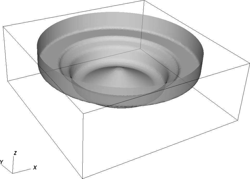
9 An example geometry of piston-bowl created using basic geometries.
Saving and reloading an EB geometry
These are the input option to save an EB geometry:
eb2.write_chk_geom=1   # defaults to 0
eb2.chkfile="chk_geom" # optional, defaults to "chk_geom"
These are the input options to read from a saved EB geometry:
eb2.geom_type="chkfile"
eb2.chkfile="chk_geom" # optional, defaults to "chk_geom"
eb2.max_grid_size=32 # optional, defaults to 64, must match the max_grid_size used to generate the EB in the first place
Setting the Covered State
By default, the state for all cells completely covered by the EB is set to the value of the initial condition of the first valid fluid cell on the base grid.
The values in the covered region do not affect values in the fluid region, but should still have valid values because some basic operations are still
carried out in the covered region, and invalid operations or NaNs may be detected during these operations if the specified values are not valid.
For debugging purposes, one may specify pelec.eb_zero_body_state = true, in which case all state variables in the covered region will be set to zero.
This will lead to NaNs when primitive variables are computed (dividing by density), but these should not propagate into fluid cells. The EB-C3 RegTest
is run with this option to ensure that covered cells do not affect fluid cells.
Problem specific inflow conditions on an EB
It is possible for the user to define problem specific conditions on an EB surface. This is done by defining an problem_eb_state function and then including pelec.eb_problem_state = 1 in the input file. An example of this is found in the EB-InflowBC case.
Warning
This is a beta feature. Currently this will only affect the calculation of the hydrodynamic fluxes so this works best for advection dominated EB conditions.
Rotational frames
Warning
PeleC has limited support for simulations using rotating frames using the single-reference-frame (SRF) method only in 3D and needs the MOL scheme when using this feature.
Single-reference-frame implementation
PeleC currently supports a non-inertial frame based implementation for rotating bodies, which are relevant for turbomachinery applications. The source terms for momentum and energy equations are applied in the non-inertial reference frame for cylindrically symmetric embedded boundaries. The total energy in the non-inertial frame is modified with the inclusion of rotatational kinetic energy:
where E is the total specific energy, e is specific internal energy, u,v,w are the velocity components, \(\omega\) is the angular velocity, and r is the distance from the rotational axis. The momentum equation includes additional source terms for Coriolis, centrifugal, and rotational acceleration:
For further details, refer to Appendix A.3 Navier-Stokes Equations in Rotating Frame of Reference in textbook Computational fluid dynamics: principles and applications by J. Blazek.
Single-reference-frame usage
Most often in turbomachinery applications, there is rotor and
a stator, which will be represented in PeleC as embedded boundaries.
The rotor will most often include blades and other components that are
not rotational symmetric like a cylindrical stator surface. This capability
will solve the governing equations in the non inertial frame where the
rotor boundary would then be a no-slip wall while the stator, which is rotationally
symmetric, will be a slip wall. Therefore, the user in this case
has to differentiate where the stator is using pelec.rf_rad parameter that
says anything beyond this radius will be a stator.
The rotational frame capability can be turned on by using these inputs:
pelec.do_rf=1  #turn on rotational frames
pelec.rf_omega=500.0 #rotational speed (rad/s)
pelec.rf_axis=2      #axis of rotation (0-x,1-y,2-z)
pelec.rf_axis_x=0.0  #x location of axis
pelec.rf_axis_y=0.0  #y location of axis
pelec.rf_axis_z=0.0  #z location of axis
pelec.rf_rad=20.0    #non-zero EB velocity beyond this radius
pelec.do_mol = 1     #rotational frames only implemented with MOL
The velocities in the plot files will be in the rotating frame.
But, one can turn on amr.derive_plot_vars to add new variables
that transform velocity back to inertial frame. These variable names
include x_velocity_if, y_velocity_if , z_velocity_if and
magvel_if.
Some example test cases
We have tested this SRF implementation using a Taylor-Couette example (see Exec/EB_TaylorCouette)
for which we obtain solutions matching the analytic solution as shown in
Figure rotational-frame-verification (a).
We have also done a comparison with the incompressible SRF solver in OpenFOAM for a
4 bladed rotor case (see Exec/EB_Rotor4Blade).
The solutions agree reasonably well, as shown in Figure rotational-frame-verification (b)
with minor differences due to the compressible formulation in PeleC.
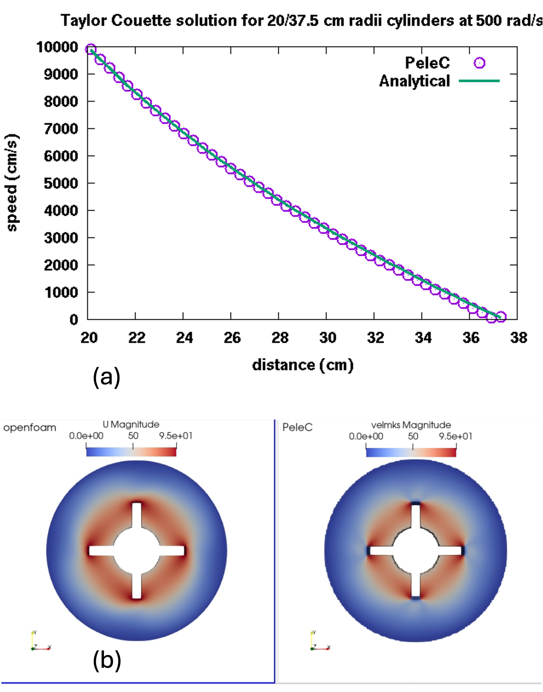
10 (a) solution to Taylor-Couette flow compared to analytic solution and (b) comparison of velocity magntiude for a 4 blade rotor case with incompressible SRF solver from OpenFOAM.