Visualization

There are several visualization tools that can be used for AMReX plotfiles. The standard tool used within the AMReX-community is Amrvis, a package developed and supported by CCSE that is designed specifically for highly efficient visualization of block-structured hierarchical AMR data. Plotfiles can also be viewed using the VisIt, ParaView, and yt packages. Particle data can be viewed using ParaView.

Amrvis

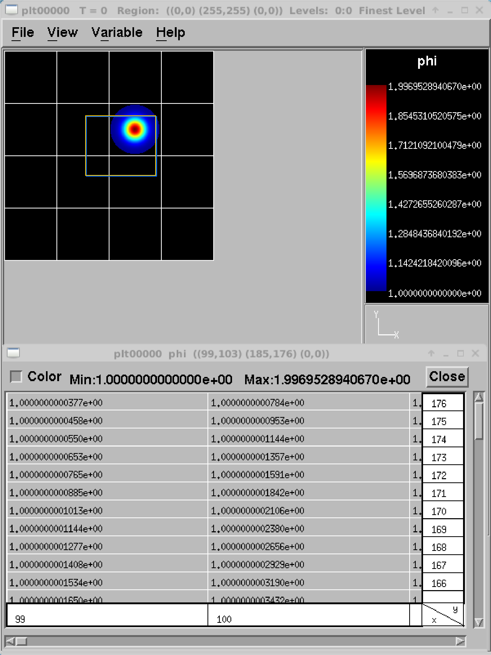
Our favorite visualization tool is Amrvis. We heartily encourage you to build the amrvis1d, amrvis2d, and amrvis3d executables, and to try using them to visualize your data. A very useful feature is View/Dataset, which allows you to actually view the numbers in a spreadsheet that is nested to reflect the AMR hierarchy – this can be handy for debugging. You can modify how many levels of data you want to see, whether you want to see the grid boxes or not, what palette you use, etc. Below are some instructions and tips for using Amrvis; you can find additional information in Amrvis/Docs/Amrvis.tex (which you can build into a pdf using pdflatex).

1. Download and build :

   git clone https://github.com/AMReX-Codes/Amrvis
   

   Then cd into Amrvis/, edit the GNUmakefile by setting COMP to the compiler suite you have.

   Type make DIM=1, make DIM=2, or make DIM=3 to build, resulting in an executable that looks like amrvis2d…ex.

   If you want to build amrvis with DIM=3, you must first download and build volpack:

   git clone https://ccse.lbl.gov/pub/Downloads/volpack.git
   

   Then cd into volpack/ and type make.

   Note: Amrvis requires the OSF/Motif libraries and headers. If you don’t have these you will need to install the development version of motif through your package manager. lesstif gives some functionality and will allow you to build the amrvis executable, but Amrvis may exhibit subtle anomalies.

   On most Linux distributions, the motif library is provided by the openmotif package, and its header files (like Xm.h) are provided by openmotif-devel. If those packages are not installed, then use the OS-specific package management tool to install them.

   You may then want to create an alias to amrvis2d, for example

   alias amrvis2d /tmp/Amrvis/amrvis2d...ex
   

2. Run the command cp Amrvis/amrvis.defaults ~/.amrvis.defaults. Then, in your copy, edit the line containing “palette” line to point to, e.g., “palette /home/username/Amrvis/Palette”. The other lines control options such as the initial field to display, the number format, widow size, etc. If there are multiple instances of the same option, the last option takes precedence.

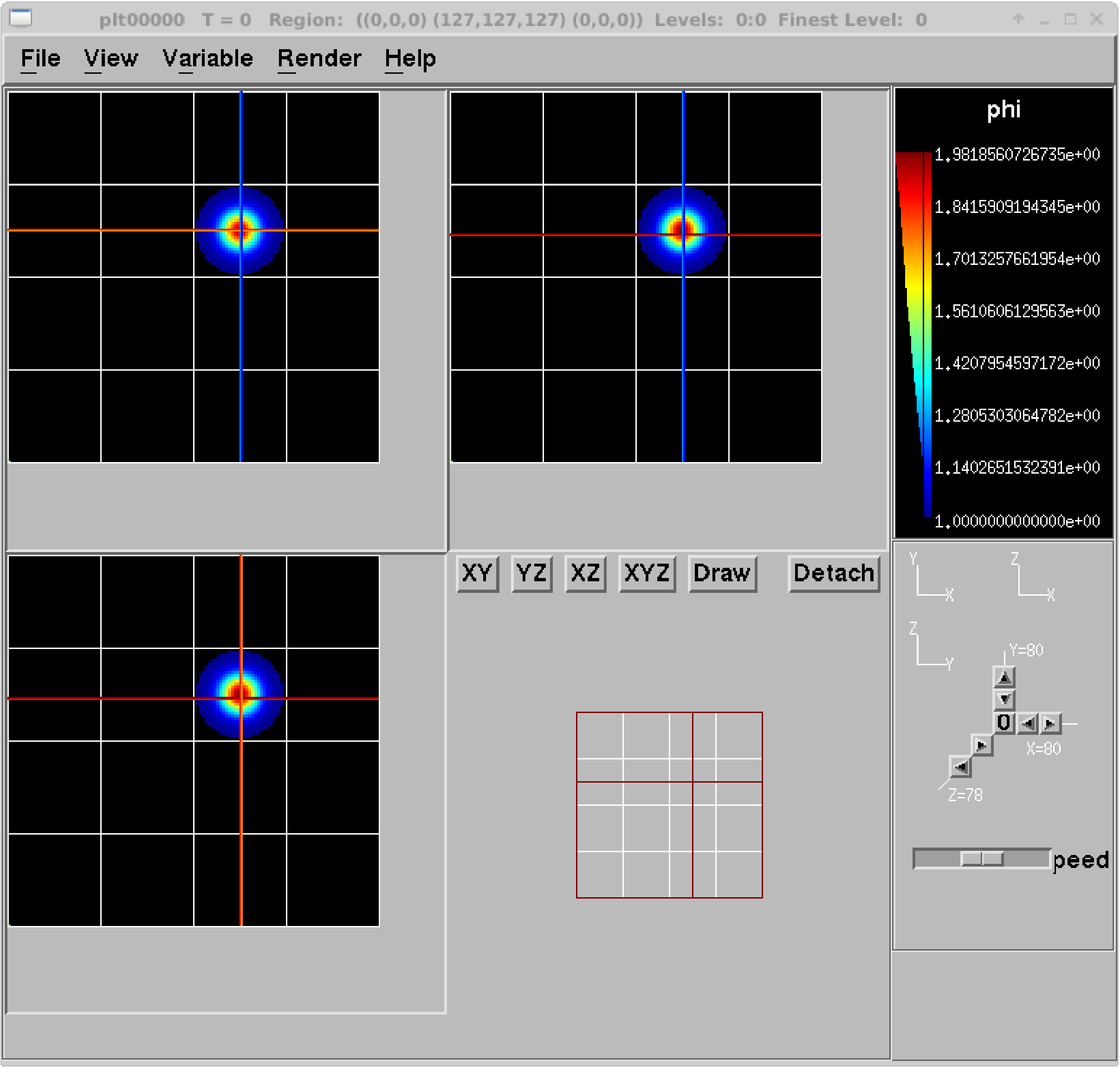
3. Generally the plotfiles have the form pltXXXXX (the plt prefix can be changed), where XXXXX is a number corresponding to the timestep the file was output. amrvis2d <filename> or amrvis3d <filename> to see a single plotfile, or for 2D data sets, amrvis2d -a plt*, which will animate the sequence of plotfiles. FArrayBoxes and MultiFabs can also be viewed with the -fab and -mf options. When opening MultiFabs, use the name of the MultiFab’s header file amrvis2d -mf MyMultiFab_H.

   You can use the “Variable” menu to change the variable. You can left-click drag a box around a region and click “View” \(\rightarrow\) “Dataset” in order to look at the actual numerical values (see 2). Or you can simply left click on a point to obtain the numerical value. You can also export the pictures in several different formats under “File/Export”. In 2D you can right and center click to get line-out plots. In 3D you can right and center click to change the planes, and the hold shift+(right or center) click to get line-out plots.

   We have created a number of routines to convert AMReX plotfile data other formats (such as matlab), but in order to properly interpret the hierarchical AMR data, each tends to have its own idiosyncrasies. If you would like to display the data in another format, please contact Marc Day (MSDay@lbl.gov) and we will point you to whatever we have that can help.

2 2D and 3D images generated using Amrvis

Building Amrvis on macOS

As previously outlined at the end of section Building with GNU Make, it is recommended to build using the homebrew package manager to install gcc. Furthermore, you will also need x11 and openmotif. These can be installed using homebrew also:

1. brew cask install xquartz

2. brew install openmotif

Note that when the GNUmakefile detects a macOS install, it assumes that dependencies are installed in the locations that Homebrew uses. Namely the /usr/local/ tree for regular dependencies and the /opt/ tree for X11.

VisIt

AMReX data can also be visualized by VisIt, an open source visualization and analysis software. To follow along with this example, first build and run the first heat equation tutorial code (see the section on XXX).

Next, download and install VisIt from https://wci.llnl.gov/simulation/computer-codes/visit. To open a single plotfile, run VisIt, then select “File” \(\rightarrow\) “Open file …”, then select the Header file associated the the plotfile of interest (e.g., plt00000/Header). Assuming you ran the simulation in 2D, here are instructions for making a simple plot:

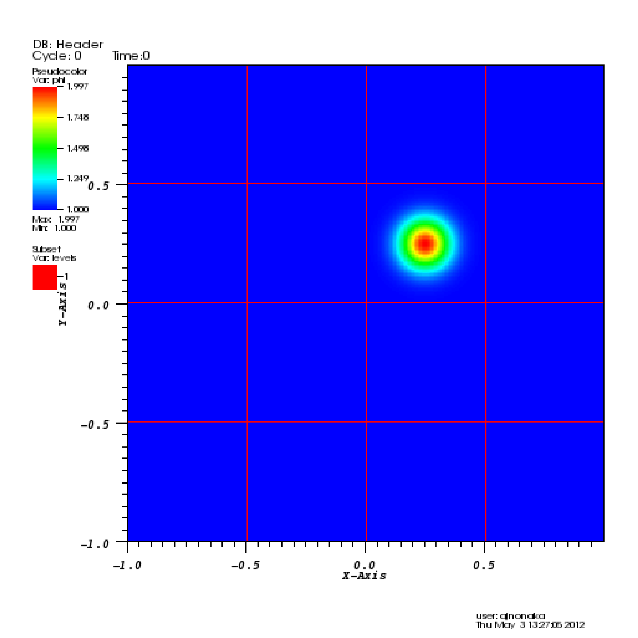
• To view the data, select “Add” \(\rightarrow\) “Pseudocolor” \(\rightarrow\) “phi”, and then select “Draw”.

• To view the grid structure (not particularly interesting yet, but when we add AMR it will be), select “ \(\rightarrow\) “subset” \(\rightarrow\) “levels”. Then double-click the text “Subset - levels”, enable the “Wireframe” option, select “Apply”, select “Dismiss”, and then select “Draw”.

• To save the image, select “File” \(\rightarrow\) “Set save options”, then customize the image format to your liking, then click “Save”.

Your image should look similar to the left side of 3.

3 : 2D (left) and 3D (right) images generated using VisIt.

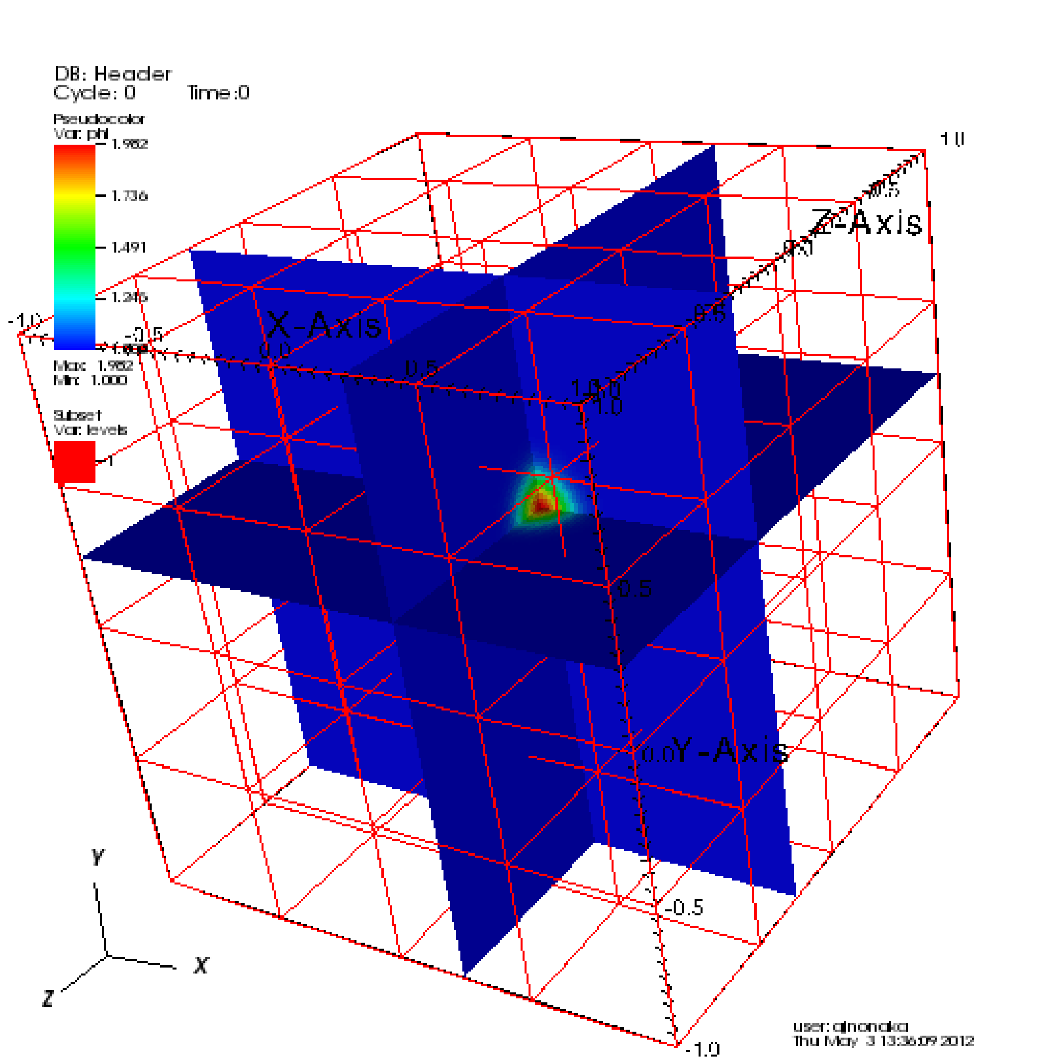
In 3D, you must apply the “Operators” \(\rightarrow\) “Slicing” \(\rightarrow\) “ThreeSlice”, with the “ThreeSlice operator attribute” set to x=0.25, y=0.25, and z=0.25. You can left-click and drag over the image to rotate the image to generate something similar to right side of 3.

To make a movie, you must first create a text file named movie.visit with a list of the Header files for the individual frames. This can most easily be done using the command:

~/amrex/Tutorials/Basic/HeatEquation_EX1_C> ls -1 plt*/Header | tee movie.visit
plt00000/Header
plt01000/Header
plt02000/Header
plt03000/Header
plt04000/Header
plt05000/Header
plt06000/Header
plt07000/Header
plt08000/Header
plt09000/Header
plt10000/Header

The next step is to run VisIt, select “File” \(\rightarrow\) “Open file …”, then select movie.visit. Create an image to your liking and press the “play” button on the VCR-like control panel to preview all the frames. To save the movie, choose “File” \(\rightarrow\) “Save movie …”, and follow the on-screen instructions.

ParaView

The open source visualization package ParaView v5.5 can be used to view 3D plotfiles, and particle data. Download the package at https://www.paraview.org/.

To open a single plotfile (for example, you could run the HeatEquation_EX1_C in 3D):

1. Run ParaView v5.5, then select “File” \(\rightarrow\) “Open”.

2. Navigate into the plotfile directory, and manually type in “Header”. ParaView will ask you about the file type – choose “Boxlib 3D Files”

3. Under the “Cell Arrays” field, select a variable (e.g., “phi”) and click “Apply”.

4. Under “Representation” select “Surface”.

5. Under “Coloring” select the variable you chose above.

6. To add planes, near the top left you will see a cube icon with a green plane slicing through it. If you hover your mouse over it, it will say “Slice”. Click that button.

7. You can play with the Plane Parameters to define a plane of data to view, as shown in 1.

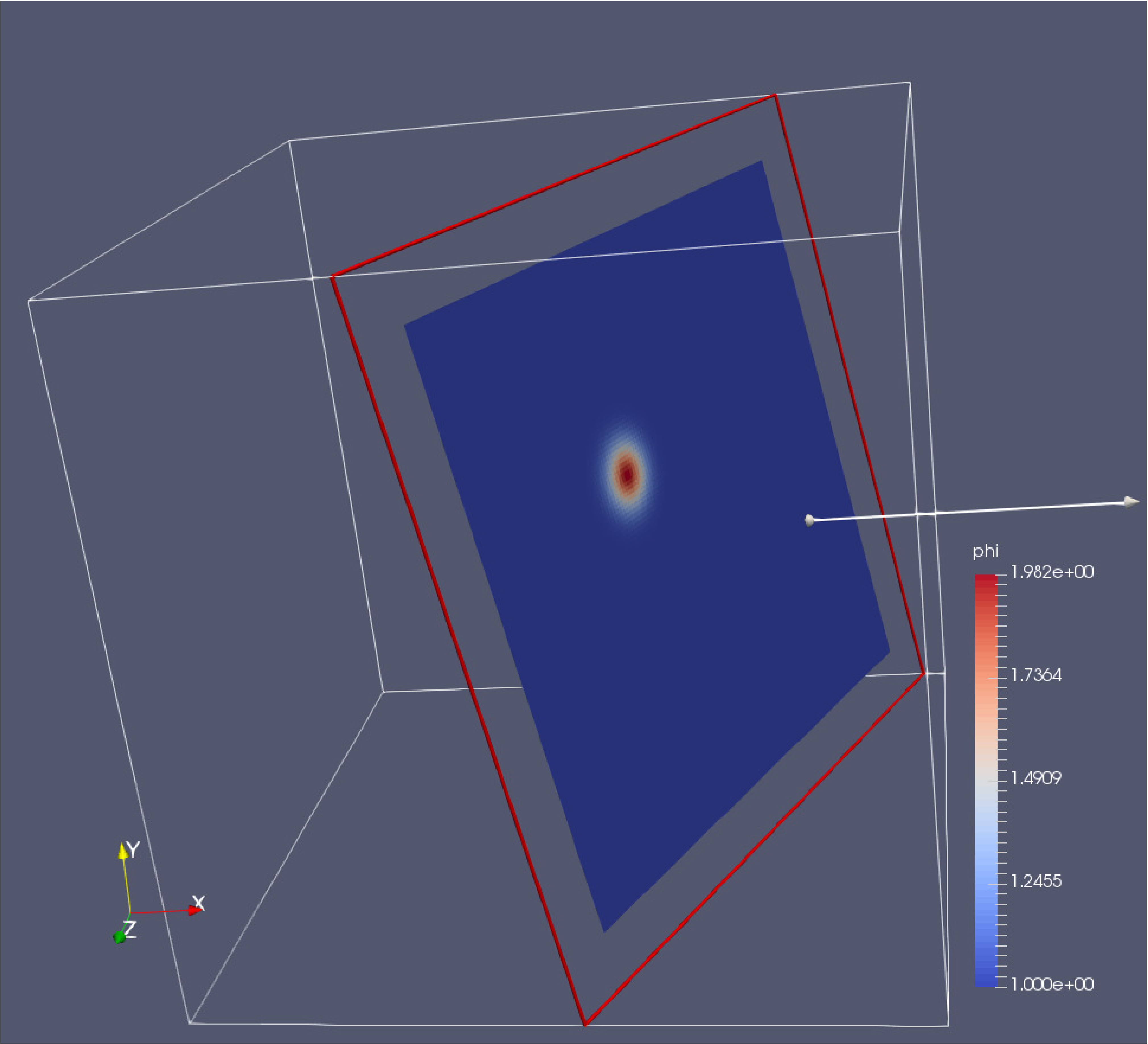
1 : Plotfile image generated with ParaView

To visualize particle data within plofile directories (for example, you could run the ShortRangeParticles example):

1. Run ParaView v5.5, and select then “File” \(\rightarrow\) “Open”. You will see a combined “plt..” group. Click on “+” to expand the group, if you want inspect the files in the group. You can select an individual plotfile directory or select a group of directories to read them a time series, as shown in 2, and click OK.

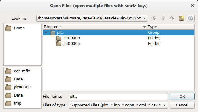
2 : File dialog in ParaView showing a group of plotfile directories selected

1. The “Properties” panel in ParaView allows you to specify the “Particle Type”, which defaults to “particles”. Using the “Properties” panel, you can also choose which point arrays to read.

2. Click “Apply” and under “Representation” select “Point Gaussian”.

3. Change the Gaussian Radius if you like. You can scroll through the frames with the VCR-like controls at the top, as shown in 3.

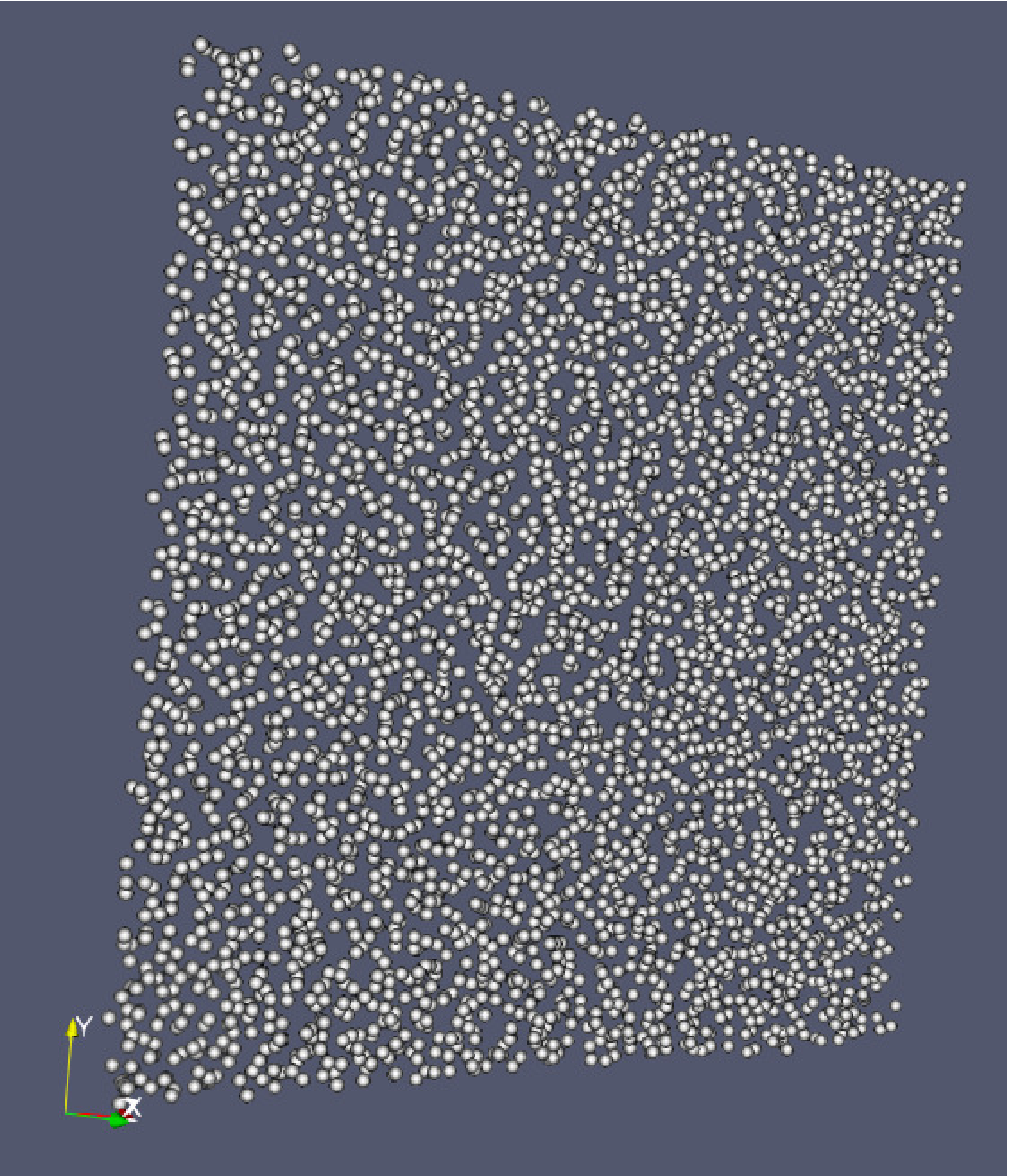
3 : Particle image generated with ParaView

yt

yt, an open source Python package available at http://yt-project.org/, can be used for analyzing and visualizing mesh and particle data generated by AMReX codes. Some of the AMReX developers are also yt project members. Below we describe how to use on both a local workstation, as well as at the NERSC HPC facility for high-throughput visualization of large data sets.

Note - AMReX datasets require yt version 3.4 or greater.

Using on a local workstation

Running yt on a local system generally provides good interactivity, but limited performance. Consequently, this configuration is best when doing exploratory visualization (e.g., experimenting with camera angles, lighting, and color schemes) of small data sets.

To use yt on an AMReX plot file, first start a Jupyter notebook or an IPython kernel, and import the yt module:

In [1]: import yt

In [2]: print(yt.__version__)
3.4-dev

Next, load a plot file; in this example we use a plot file from the Nyx cosmology application:

In [3]: ds = yt.load("plt00401")
yt : [INFO     ] 2017-05-23 10:03:56,182 Parameters: current_time              = 0.00605694344696544
yt : [INFO     ] 2017-05-23 10:03:56,182 Parameters: domain_dimensions         = [128 128 128]
yt : [INFO     ] 2017-05-23 10:03:56,182 Parameters: domain_left_edge          = [ 0.  0.  0.]
yt : [INFO     ] 2017-05-23 10:03:56,183 Parameters: domain_right_edge         = [ 14.24501  14.24501  14.24501]

In [4]: ds.field_list
Out[4]:
[('DM', 'particle_mass'),
 ('DM', 'particle_position_x'),
 ('DM', 'particle_position_y'),
 ('DM', 'particle_position_z'),
 ('DM', 'particle_velocity_x'),
 ('DM', 'particle_velocity_y'),
 ('DM', 'particle_velocity_z'),
 ('all', 'particle_mass'),
 ('all', 'particle_position_x'),
 ('all', 'particle_position_y'),
 ('all', 'particle_position_z'),
 ('all', 'particle_velocity_x'),
 ('all', 'particle_velocity_y'),
 ('all', 'particle_velocity_z'),
 ('boxlib', 'density'),
 ('boxlib', 'particle_mass_density')]

From here one can make slice plots, 3-D volume renderings, etc. An example of the slice plot feature is shown below:

In [9]: slc = yt.SlicePlot(ds, "z", "density")
yt : [INFO     ] 2017-05-23 10:08:25,358 xlim = 0.000000 14.245010
yt : [INFO     ] 2017-05-23 10:08:25,358 ylim = 0.000000 14.245010
yt : [INFO     ] 2017-05-23 10:08:25,359 xlim = 0.000000 14.245010
yt : [INFO     ] 2017-05-23 10:08:25,359 ylim = 0.000000 14.245010

In [10]: slc.show()

In [11]: slc.save()
yt : [INFO     ] 2017-05-23 10:08:34,021 Saving plot plt00401_Slice_z_density.png
Out[11]: ['plt00401_Slice_z_density.png']

The resulting image is 4. One can also make volume renderings with ; an example is show below:

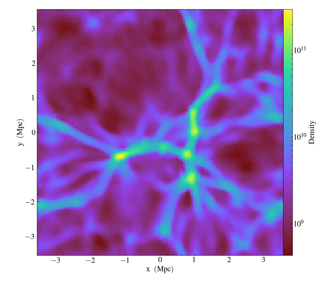
4 : Slice plot of \(128^3\) Nyx simulation using yt.

In [12]: sc = yt.create_scene(ds, field="density", lens_type="perspective")

In [13]: source = sc[0]

In [14]: source.tfh.set_bounds((1e8, 1e15))

In [15]: source.tfh.set_log(True)

In [16]: source.tfh.grey_opacity = True

In [17]: sc.show()
<Scene Object>:
Sources:
    source_00: <Volume Source>:YTRegion (plt00401): , center=[  1.09888770e+25   1.09888770e+25   1.09888770e+25] cm, left_edge=[ 0.  0.  0.] cm, right_edge=[  2.19777540e+25   2.19777540e+25   2.19777540e+25] cm transfer_function:None
Camera:
    <Camera Object>:
    position:[ 14.24501  14.24501  14.24501] code_length
    focus:[ 7.122505  7.122505  7.122505] code_length
    north_vector:[ 0.81649658 -0.40824829 -0.40824829]
    width:[ 21.367515  21.367515  21.367515] code_length
    light:None
    resolution:(512, 512)
Lens: <Lens Object>:
    lens_type:perspective
    viewpoint:[ 0.95423473  0.95423473  0.95423473] code_length

In [19]: sc.save()
yt : [INFO     ] 2017-05-23 10:15:07,825 Rendering scene (Can take a while).
yt : [INFO     ] 2017-05-23 10:15:07,825 Creating volume
yt : [INFO     ] 2017-05-23 10:15:07,996 Creating transfer function
yt : [INFO     ] 2017-05-23 10:15:07,997 Calculating data bounds. This may take a while.
Set the TransferFunctionHelper.bounds to avoid this.
yt : [INFO     ] 2017-05-23 10:15:16,471 Saving render plt00401_Render_density.png

The output of this is 5.

5 Volume rendering of \(128^3\) Nyx simulation using yt. This corresponds to the same plot file used to generate the slice plot in 4.

Using yt at NERSC (under development)

Because yt is Python-based, it is portable and can be used in many software environments. Here we focus on yt’s capabilities at NERSC, which provides resources for performing both interactive and batch queue-based visualization and analysis of AMReX data. Coupled with yt’s MPI and OpenMP parallelization capabilities, this can enable high-throughput visualization and analysis workflows.

Interactive yt with Jupyter notebooks

Unlike VisIt (see the section on VisIt), yt has no client-server interface. Such an interface is often crucial when one has large data sets generated on a remote system, but wishes to visualize the data on a local workstation. Both copying the data between the two systems, as well as visualizing the data itself on a workstation, can be prohibitively slow.

Fortunately, NERSC has implemented several resources which allow one to interact with yt remotely, emulating a client-server model. In particular, NERSC now hosts Jupyter notebooks which run IPython kernels on the Cori system; this provides users access to the $HOME, /project, and $SCRATCH file systems from a web browser-based Jupyter notebook. *Please note that Jupyter hosting at NERSC is still under development, and the environment may change without notice.*

NERSC also provides Anaconda Python, which allows users to create their own customizable Python environments. It is recommended to install yt in such an environment. One can do so with the following example:

user@cori10:~> module load python/3.5-anaconda
user@cori10:~> conda create -p $HOME/yt-conda numpy
user@cori10:~> source activate $HOME/yt-conda
(/global/homes/u/user/yt-conda/) user@cori10:~> pip install yt

More information about Anaconda Python at NERSC is here: http://www.nersc.gov/users/data-analytics/data-analytics/python/anaconda-python/.

One can then configure this Anaconda environment to run in a Jupyter notebook hosted on the Cori system. Currently this is available in two places: on https://ipython.nersc.gov, and on https://jupyter-dev.nersc.gov. The latter likely reflects what the stable, production environment for Jupyter notebooks will look like at NERSC, but it is still under development and subject to change. To load this custom Python kernel in a Jupyter notebook, follow the instructions at this URL under the “Custom Kernels” heading: http://www.nersc.gov/users/data-analytics/data-analytics/web-applications-for-data-analytics. After writing the appropriate kernel.json file, the custom kernel will appear as an available Jupyter notebook. Then one can interactively visualize AMReX plot files in the web browser. 1

Parallel

Besides the benefit of no longer needing to move data back and forth between NERSC and one’s local workstation to do visualization and analysis, an additional feature of yt which takes advantage of the computational resources at NERSC is its parallelization capabilities. yt supports both MPI- and OpenMP-based parallelization of various tasks, which are discussed here: http://yt-project.org/doc/analyzing/parallel_computation.html.

Configuring yt for MPI parallelization at NERSC is a more complex task than discussed in the official yt documentation; the command pip install mpi4py is not sufficient. Rather, one must compile mpi4py from source using the Cray compiler wrappers cc, CC, and ftn on Cori. Instructions for compiling mpi4py at NERSC are provided here: http://www.nersc.gov/users/data-analytics/data-analytics/python/anaconda-python/#toc-anchor-3. After mpi4py has been compiled, one can use the regular Python interpreter in the Anaconda environment as normal; when executing yt operations which support MPI parallelization, the multiple MPI processes will spawn automatically.

Although several components of yt support MPI parallelization, a few are particularly useful:

• Time series analysis. Often one runs a simulation for many time steps and periodically writes plot files to disk for visualization and post-processing. yt supports parallelization over time series data via the DatasetSeries object. yt can iterate over a DatasetSeries in parallel, with different MPI processes operating on different elements of the series. This page provides more documentation: http://yt-project.org/doc/analyzing/time_series_analysis.html#time-series-analysis.

• Volume rendering. yt implements spatial decomposition among MPI processes for volume rendering procedures, which can be computationally expensive. Note that yt also implements OpenMP parallelization in volume rendering, and so one can execute volume rendering with a hybrid MPI+OpenMP approach. See this URL for more detail: http://yt-project.org/doc/visualizing/volume_rendering.html?highlight=openmp#openmp-parallelization.

• Generic parallelization over multiple objects. Sometimes one wishes to loop over a series which is not a DatasetSeries, e.g., performing translational or rotational operations on a camera to make a volume rendering in which the field of view moves through the simulation. In this case, one is applying a set of operations on a single object (a single plot file), rather than over a time series of data. For this workflow, yt provides the parallel_objects() function. See this URL for more details: http://yt-project.org/doc/analyzing/parallel_computation.html#parallelizing-over-multiple-objects.

  An example of MPI parallelization in yt is shown below, where one animates a time series of plot files from an IAMR simulation while revolving the camera such that it completes two full revolutions over the span of the animation:

  import yt
  import glob
  import numpy as np
  
  yt.enable_parallelism()
  
  base_dir1 = '/global/cscratch1/sd/user/Nyx_run_p1'
  base_dir2 = '/global/cscratch1/sd/user/Nyx_run_p2'
  base_dir3 = '/global/cscratch1/sd/user/Nyx_run_p3'
  
  glob1 = glob.glob(base_dir1 + '/plt*')
  glob2 = glob.glob(base_dir2 + '/plt*')
  glob3 = glob.glob(base_dir3 + '/plt*')
  
  files = sorted(glob1 + glob2 + glob3)
  
  ts = yt.DatasetSeries(files, parallel=True)
  
  frame = 0
  num_frames = len(ts)
  num_revol = 2
  
  slices = np.arange(len(ts))
  
  for i in yt.parallel_objects(slices):
      sc = yt.create_scene(ts[i], lens_type='perspective', field='z_velocity')
  
      source = sc[0]
      source.tfh.set_bounds((1e-2, 9e+0))
      source.tfh.set_log(False)
      source.tfh.grey_opacity = False
  
      cam = sc.camera
  
      cam.rotate(num_revol*(2.0*np.pi)*(i/num_frames),
                 rot_center=np.array([0.0, 0.0, 0.0]))
  
      sc.save(sigma_clip=5.0)
  

  When executed on 4 CPUs on a Haswell node of Cori, the output looks like the following:

  user@nid00009:~/yt_vis/> srun -n 4 -c 2 --cpu_bind=cores python make_yt_movie.py
  yt : [INFO     ] 2017-05-23 16:51:33,565 Global parallel computation enabled: 0 / 4
  yt : [INFO     ] 2017-05-23 16:51:33,565 Global parallel computation enabled: 2 / 4
  yt : [INFO     ] 2017-05-23 16:51:33,566 Global parallel computation enabled: 1 / 4
  yt : [INFO     ] 2017-05-23 16:51:33,566 Global parallel computation enabled: 3 / 4
  P003 yt : [INFO     ] 2017-05-23 16:51:33,957 Parameters: current_time              = 0.103169376949795
  P003 yt : [INFO     ] 2017-05-23 16:51:33,957 Parameters: domain_dimensions         = [128 128 128]
  P003 yt : [INFO     ] 2017-05-23 16:51:33,957 Parameters: domain_left_edge          = [ 0.  0.  0.]
  P003 yt : [INFO     ] 2017-05-23 16:51:33,958 Parameters: domain_right_edge         = [ 6.28318531  6.28318531  6.28318531]
  P000 yt : [INFO     ] 2017-05-23 16:51:33,969 Parameters: current_time              = 0.0
  P000 yt : [INFO     ] 2017-05-23 16:51:33,969 Parameters: domain_dimensions         = [128 128 128]
  P002 yt : [INFO     ] 2017-05-23 16:51:33,969 Parameters: current_time              = 0.0687808060674485
  P000 yt : [INFO     ] 2017-05-23 16:51:33,969 Parameters: domain_left_edge          = [ 0.  0.  0.]
  P002 yt : [INFO     ] 2017-05-23 16:51:33,969 Parameters: domain_dimensions         = [128 128 128]
  P000 yt : [INFO     ] 2017-05-23 16:51:33,970 Parameters: domain_right_edge         = [ 6.28318531  6.28318531  6.28318531]
  P002 yt : [INFO     ] 2017-05-23 16:51:33,970 Parameters: domain_left_edge          = [ 0.  0.  0.]
  P002 yt : [INFO     ] 2017-05-23 16:51:33,970 Parameters: domain_right_edge         = [ 6.28318531  6.28318531  6.28318531]
  P001 yt : [INFO     ] 2017-05-23 16:51:33,973 Parameters: current_time              = 0.0343922351851018
  P001 yt : [INFO     ] 2017-05-23 16:51:33,973 Parameters: domain_dimensions         = [128 128 128]
  P001 yt : [INFO     ] 2017-05-23 16:51:33,974 Parameters: domain_left_edge          = [ 0.  0.  0.]
  P001 yt : [INFO     ] 2017-05-23 16:51:33,974 Parameters: domain_right_edge         = [ 6.28318531  6.28318531  6.28318531]
  P000 yt : [INFO     ] 2017-05-23 16:51:34,589 Rendering scene (Can take a while).
  P000 yt : [INFO     ] 2017-05-23 16:51:34,590 Creating volume
  P003 yt : [INFO     ] 2017-05-23 16:51:34,592 Rendering scene (Can take a while).
  P002 yt : [INFO     ] 2017-05-23 16:51:34,592 Rendering scene (Can take a while).
  P003 yt : [INFO     ] 2017-05-23 16:51:34,593 Creating volume
  P002 yt : [INFO     ] 2017-05-23 16:51:34,593 Creating volume
  P001 yt : [INFO     ] 2017-05-23 16:51:34,606 Rendering scene (Can take a while).
  P001 yt : [INFO     ] 2017-05-23 16:51:34,607 Creating volume
  

  Because the parallel_objects() function transforms the loop into a data-parallel problem, this procedure strong scales nearly perfectly to an arbitrarily large number of MPI processes, allowing for rapid rendering of large time series of data.

1

It is convenient to use the magic command %matplotlib inline in order to render matplotlib figures in the same browser window as the notebook, as opposed to displaying it as a new window.

SENSEI

SENSEI is a light weight framework for in situ data analysis. SENSEI’s data model and API provide uniform access to and run time selection of a diverse set of visualization and analysis back ends including VisIt Libsim, ParaView Catalyst, VTK-m, Ascent, ADIOS, Yt, and Python.

System Architecture

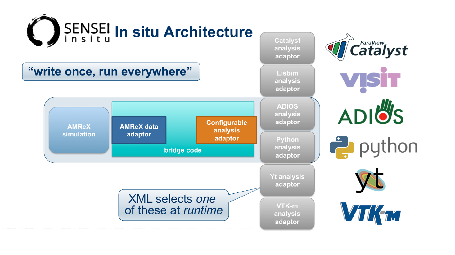
6 SENSEI’s in situ architecture enables use of a diverse of back ends which can be selected at run time via an XML configuration file

The three major architectural components in SENSEI are data adaptors which present simulation data in SENSEI’s data model, analysis adaptors which present the back end data consumers to the simulation, and bridge code from which the simulation manages adaptors and periodically pushes data through the system. SENSEI comes equipped with a number of analysis adaptors enabling use of popular analysis and visualization libraries such as VisIt Libsim, ParaView Catalyst, Python, and ADIOS to name a few. AMReX contains SENSEI data adaptors and bridge code making it easy to use in AMReX based simulation codes.

SENSEI provides a configurable analysis adaptor which uses an XML file to select and configure one or more back ends at run time. Run time selection of the back end via XML means one user can access Catalyst, another Libsim, yet another Python with no changes to the code. This is depicted in figure 6. On the left side of the figure AMReX produces data, the bridge code pushes the data through the configurable analysis adaptor to the back end that was selected at run time.

AMReX Integration

AMReX codes based on amrex::Amr can use SENSEI simply by enabling it in the build and run via ParmParse parameters. AMReX codes based on amrex::AmrMesh need to additionally invoke the bridge code in amrex::AmrMeshInSituBridge.

Compiling with GNU Make

For codes making use of AMReX’s build system add the following variable to the code’s main GNUmakefile.

USE_SENSEI_INSITU = TRUE

When set, AMReX’s make files will query environment variables for the lists of compiler and linker flags, include directories, and link libraries. These lists can be quite elaborate when using more sophisticated back ends, and are best set automatically using the sensei_config command line tool that should be installed with SENSEI. Prior to invoking make use the following command to set these variables:

source sensei_config

Typically, the sensei_config tool is in the users PATH after loading the desired SENSEI module. After configuring the build environment with sensei_config, proceed as usual.

make -j4 -f GNUmakefile

ParmParse Configuration

Once an AMReX code has been compiled with SENSEI features enabled, it will need to be enabled and configured at runtime. This is done using ParmParse input file. The following 3 ParmParse parameters are used:

sensei.enabled = 1
sensei.config = render_iso_catalyst_2d.xml
sensei.frequency = 2

sensei.enabled turns SENSEI on or off. sensei.config points to the SENSEI XML file which selects and configures the desired back end. sensei.frequency controls the number of level 0 time steps in between SENSEI processing.

Back-end Selection and Configuration

The back end is selected and configured at run time using the SENSEI XML file. The XML sets parameters specific to SENSEI and to the chosen back end. Many of the back ends have sophisticated configuration mechanisms which SENSEI makes use of. For example the following XML configuration was used on NERSC’s Cori with IAMR to render 10 iso surfaces, shown in figure 7, using VisIt Libsim.

<sensei>
  <analysis type="libsim" frequency="1" mode="batch"
    visitdir="/usr/common/software/sensei/visit"
    session="rt_sensei_configs/visit_rt_contour_alpha_10.session"
    image-filename="rt_contour_%ts" image-width="1555" image-height="815"
    image-format="png" enabled="1"/>
</sensei>

The session attribute names a session file that contains VisIt specific runtime configuration. The session file is generated using VisIt GUI on a representative dataset. Usually this data set is generated in a low resolution run of the desired simulation.

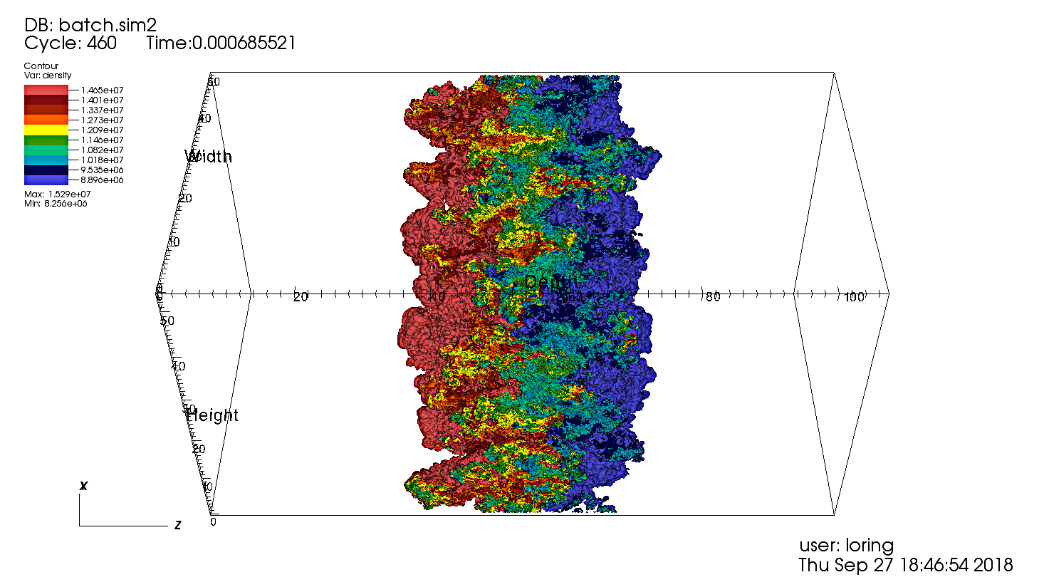
7 SENSEI-Libsim in situ visualization of a Raleigh-Taylor instability computed by IAMR on NERSC Cori using 2048 cores.

The same run and visualization was repeated using ParaView Catalyst, shown in figure 8, by providing the following XML configuration.

<sensei>
  <analysis type="catalyst" pipeline="pythonscript"
    filename="rt_sensei_configs/rt_contour.py" enabled="1" />
</sensei>

Here the filename attribute is used to pass Catalyst a Catalyst specific configuration that was generated using the ParaView GUI on a representative dataset.

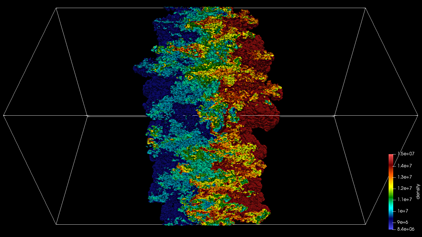
8 SENSEI-Catalyst in situ visualization of a Raleigh-Taylor instability computed by IAMR on NERSC Cori using 2048 cores.

Obtaining SENSEI

SENSEI is hosted on Kitware’s Gitlab site at https://gitlab.kitware.com/sensei/sensei It’s best to checkout the latest release rather than working on the master branch.

To ease the burden of wrangling back end installs SENSEI provides two platforms with all dependencies pre-installed, a VirtualBox VM, and a NERSC Cori deployment. New users are encouraged to experiment with one of these.

SENSEI VM

The SENSEI VM comes with all of SENSEI’s dependencies and the major back ends such as VisIt and ParaView installed. The VM is the easiest way to test things out. It also can be used to see how installs were done and the environment configured.

NERSC Cori

SENSEI is deployed at NERSC on Cori. The NERSC deployment includes the major back ends such as ParaView Catalyst, VisIt Libsim, and Python.

AmrLevel Tutorial with Catalyst

The following steps show how to run the tutorial with ParaView Catalyst. The simulation will periodically write images during the run.

ssh cori.nersc.gov
cd $SCRATCH
git clone https://github.com/AMReX-Codes/amrex.git
cd amrex/Tutorials/Amr/Advection_AmrLevel/Exec/SingleVortex
module use /usr/common/software/sensei/modulefiles
module load sensei/2.1.0-catalyst-shared
source sensei_config
vim GNUmakefile
# USE_SENSEI_INSITU=TRUE
make -j4 -f GNUmakefile
vim inputs
# sensei.enabled=1
# sensei.config=sensei/render_iso_catalyst_2d.xml
salloc -C haswell -N 1 -t 00:30:00 -q debug
cd $SCRATCH/amrex/Tutorials/Amr/Advection_AmrLevel/Exec/SingleVortex
./main2d.gnu.haswell.MPI.ex inputs

AmrLevel Tutorial with Libsim

The following steps show how to run the tutorial with VisIt Libsim. The simulation will periodically write images during the run.

ssh cori.nersc.gov
cd $SCRATCH
git clone https://github.com/AMReX-Codes/amrex.git
cd amrex/Tutorials/Amr/Advection_AmrLevel/Exec/SingleVortex
module use /usr/common/software/sensei/modulefiles
module load sensei/2.1.0-libsim-shared
source sensei_config
vim GNUmakefile
# USE_SENSEI_INSITU=TRUE
make -j4 -f GNUmakefile
vim inputs
# sensei.enabled=1
# sensei.config=sensei/render_iso_libsim_2d.xml
salloc -C haswell -N 1 -t 00:30:00 -q debug
./main2d.gnu.haswell.MPI.ex inputs