Spray Flags and Inputs

In the GNUmakefile, specify USE_PARTICLES = TRUE and SPRAY_FUEL_NUM = N where N is the number of liquid species being used in the simulation.
Depending on the gas phase solver, spray solving functionality can be turned on in the input file using pelec.do_spray_particles = 1 or peleLM.do_spray_particles = 1.
The units for PeleLM and PeleLMeX are MKS while the units for PeleC are CGS. This is the same for the spray inputs. E.g. when running a spray simulation coupled with PeleC, the units for particles.fuel_cp must be in erg/g.
There are many required particles. flags in the input file. For demonstration purposes, 2 liquid species of NC7H16 and NC10H22 will be used.
- The liquid fuel species names are specified using particles.fuel_species = NC7H16 NC10H22. The number of fuel species listed must match SPRAY_FUEL_NUM.
- Many values must be specified on a per-species basis. Following the current example, one would have to specify particles.NC7H16_crit_temp = 540. and particles.NC10H22_crit_temp = 617. to set a critical temperature of 540 K for NC7H16 and 617 K for NC10H22.
- Although this is not required or typical, if the evaporated mass should contribute to a different gas phase species than what is modeled in the liquid phase, use particles.dep_fuel_species. For example, if we wanted the evaporated mass from both liquid species to contribute to a different species called SP3, we would put particles.dep_fuel_species = SP3 SP3. All species specified must be present in the chemistry transport and thermodynamic data.
The following table lists other inputs related to particles., where SP will refer to a fuel species name

Input	Description	Required	Default Value
`fuel_species`	Names of liquid species	Yes	None
`dep_fuel_species`	Name of gas phase species to contribute	Yes	Inputs to `fuel_species`
`fuel_ref_temp`	Liquid reference temperature	Yes	None
`SP_crit_temp`	Critical temperature	Yes	None
`SP_boil_temp`	Boiling temperature at atmospheric pressure	Yes	None
`SP_cp`	Liquid \(c_p\) at reference temperature	Yes	None
`SP_latent`	Latent heat at reference temperature	Yes	None
`SP_rho`	Liquid density	Yes	None
`SP_lambda`	Liquid thermal conductivity (currently unused)	No
`SP_mu`	Liquid dynamic viscosity (currently unused)	No
`mom_transfer`	Couple momentum with gas phase	No	`1`
`mass_transfer`	Evaporate mass and exchange heat with gas phase	No	`1`
`fixed_parts`	Fix particles in space	No	`0`
`parcel_size`	\(N_{d}\); Number of droplets per parcel	No	`1.`
`write_ascii_files`	Output ascii files of spray data	No	`0`
`cfl`	Particle CFL number for limiting time step	No	`0.5`
`init_file`	Ascii file name to initialize droplets	No	Empty

If an Antoine fit for saturation pressure is used, it must be specified for individual species,
```
particles.SP_psat = 4.07857 1501.268 -78.67 1.E5
```
where the numbers represent \(a\), \(b\), \(c\), and \(d\), respectively in:

\[p_{\rm{sat}}(T) = d 10^{a - b / (T + c)}\]
- If no fit is provided, the saturation pressure is estimated using the Clasius-Clapeyron relation; see
Temperature based fits for liquid density, thermal conductivity, and dynamic viscosity can be used; these can be specified as
```
particles.SP_rho = 10.42 -5.222 1.152E-2 4.123E-7
particles.SP_lambda = 7.243 1.223 4.223E-8 8.224E-9
particles.SP_mu = 7.243 1.223 4.223E-8 8.224E-9
```
where the numbers respresent \(a\), \(b\), \(c\), and \(d\), respectively in:

\[ \begin{align}\begin{aligned}\rho_L \,, \lambda_L = a + b T + c T^2 + d T^3\\\mu_L = a + b / T + c / T^2 + d / T^3\end{aligned}\end{align} \]

If only a single value is provided, \(a\) is assigned to that value and the other coefficients are set to zero, effectively using a constant value for the parameters.

Spray Injection

Templates to facilitate and simplify spray injection are available in PeleMP. To use them, changes must be made to the input and SprayParticlesInitInsert.cpp files. Inputs related to injection use the spray. parser name. To create a jet in the domain, modify the InitSprayParticles() function in SprayParticleInitInsert.cpp. Here is an example:

void
SprayParticleContainer::InitSprayParticles(
const bool init_parts, ProbParm const& prob_parm)
{
  amrex::ignore_unused(prob_parm);
  int num_jets = 1;
  m_sprayJets.resize(num_jets);
  std::string jet_name = "jet1";
  m_sprayJets[0] = std::make_unique<SprayJet>(jet_name, Geom(0));
  return;
}

This creates a single jet that is named jet1. This name will be used in the input file to reference this particular jet. For example, to set the location of the jet center for jet1, the following should be included in the input file,

spray.jet1.jet_cent = 0. 0. 0.

No two jets may have the same name. If an injector is constructed using only a name and geometry, the injection parameters are read from the input file. Here is a list of injection related inputs:

Input	Description	Required
`jet_cent`	Jet center location	Yes
`jet_norm`	Jet normal direction	Yes
`jet_vel`	Jet velocity magnitude	Yes
`jet_dia`	Jet diameter	Yes
`spread_angle`	\(\theta_J\); Full spread angle in degrees from the jet normal direction; droplets vary from \([-\theta_J/2,\theta_J/2]\)	Yes
`T`	Temperature of the injected liquid	Yes
`Y`	Mass fractions of the injected liquid based on `particles.fuel_species`	Yes, if `SPRAY_FUEL_NUM` > 1
`mass_flow_rate`	\(\dot{m}_{\rm{inj}}\); Mass flow rate of the jet	Yes
`hollow_spray`	Sets hollow cone injection with angle \(\theta_J/2\)	No (Default: 0)
`hollow_spread`	\(\theta_h\); Adds spread to hollow cone \(\theta_J/2\pm \theta_h\)	No (Default: 0)
`swirl_angle`	\(\phi_S\); Adds a swirling component along azimuthal direction	No (Default: 0)
`start_time` and `end_time`	Beginning and end time for jet	No
`dist_type`	Droplet diameter distribution type: `Uniform`, `Normal`, `LogNormal`, `Weibull`, `ChiSquared`	Yes

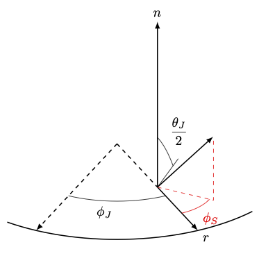
_images/inject_transform.png — Demonstration of injection angles. \(\phi_J\) varies uniformly from \([0, 2 \pi]\)

Care must be taken to ensure the amount of mass injected during a time step matches the desired mass flow rate. For smaller time steps, the risk of over-injecting mass increases. To mitigate this issue, each jet accounts for three values: \(N_{P,\min}\), \(m_{\rm{acc}}\), and \(t_{\rm{acc}}\) (labeled in the code as m_minParcel, m_sumInjMass, and m_sumInjTime, respectively). \(N_{P,\min}\) is the minimum number of parcels that must be injected over the course of an injection event; this must be greater than or equal to one. \(m_{\rm{acc}}\) is the amount of uninjected mass accumulated over the time period \(t_{\rm{acc}}\). The injection routine steps are as follows:

The injected mass for the current time step is computed using the desired mass flow rate, \(\dot{m}_{\rm{inj}}\) and the current time step

\[m_{\rm{inj}} = \dot{m}_{\rm{inj}} \Delta t + m_{\rm{acc}}\]
The time period for the current injection event is computed using

\[t_{\rm{inj}} = \Delta t + t_{\rm{acc}}\]
Using the average mass of an injected parcel, \(N_{d} m_{d,\rm{avg}}\), the estimated number of injected parcels is computed

\[N_{P, \rm{inj}} = m_{\rm{inj}} / (N_{d} m_{d, \rm{avg}})\]

If \(N_{P, \rm{inj}} < N_{P, \min}\), the mass and time is accumulated as \(m_{\rm{acc}} = m_{\rm{inj}}\) and \(t_{\rm{acc}} = t_{\rm{inj}}\) and no injection occurs this time step.

Otherwise, \(m_{\rm{inj}}\) mass is injected and convected over time \(t_{\rm{inj}}\) and \(m_{\rm{acc}}\) and \(t_{\rm{acc}}\) are reset.

If injection occurs, the amount of mass injected, \(m_{\rm{actual}}\), is summed and compared with the desired mass flow rate. If \(m_{\rm{actual}} / t_{\rm{inj}} - \dot{m}_{\rm{inj}} > 0.05 \dot{m}_{\rm{inj}}\), then \(N_{P,\min}\) is increased by one to reduce the liklihood of over-injecting in the future. A balance is necessary: the higher the minimum number of parcels, the less likely to over-inject mass but the number of time steps between injections can potentially grow as well.