Performances
PeleLMeX development was driven by the need to create a simulation code efficiently leveraging the computational power of ExaScale super-computers. As mentioned earlier, PeleLMeX is built upon the AMR library AMReX and inherits most of its High Performance Computing features.
PeleLMeX parallel paradigm is based on an MPI+`X` approach, where X can be OpenMP, or any of CUDA, HIP or SYCL, for Nvidia, AMD and Intel GPUs vendor, respectively. The actual performances gain of using accelerator within PeleLMeX is a moving target as both hardware and software are continuously improving. In the following we demonstrate the gain at a given time (specified and subject to updates) and on selected platforms.
Single node performances: FlameSheet case
Case description
The simple case of a laminar premixed flame with harmonic perturbation can be found in Exec/RegTests/FlameSheet. For the following test, the mixture is composed of dodecane and air at ambient temperature and pressure. The chemical mechanism used consist of 35 transported species and 18 species assumed in Quqsi-Steady State (QSS) and the Simple transport model with the Fuego EOS is used:
Chemistry_Model = dodecane_lu_qss
Eos_Model       = Fuego
Transport_Model = Simple
The initial solution is provided from a Cantera simulation and averaged on the cartesian grid. The input file Exec/RegTests/FlameSheet/inputs.3d_DodecaneQSS is used, with modifications detailed hereafter. Simulations are conducted at a fixed time step size for 16 steps, bypassing the initial reduction of the time step size usually employed to remove artifacts from the initial data:
amr.max_step = 16
amr.dt_shrink = 1.0
amr.fixed_dt = 2.5e-7
Additionally, unless otherwise specified, all the tests on GPUs are conducted using the MAGMA dense-direct solver to solve for the Newton direction within CVODE’s non-linear integration.
cvode.solve_type = magma_direct
and the dense direct analytical Jacobian solver on CPUs:
cvode.solve_type = denseAJ_direct
The actual number of cells in each direction and the number of levels will depends on the amount of memory available on the different platform and will be specified later on.
Results on Perlmutter (NERSC)
Perlmutter’s GPU nodes consists of a single AMD EPYC 7763 (Milan) CPU connected to 4 NVIDIA A100 GPUs. The CPU nodes consists of two of the same AMD EPYC, 64-cores CPUs. When running on the GPU node, PeleLMeX will use 4 MPI ranks with each access to one A100, while when running on a CPU node, we will use 128 MPI-ranks.
The FlameSheet case is ran using 2 levels of refinement (3 levels total) and the following domain size and cell count:
geometry.prob_lo     = 0.0 0.0 0.0        # x_lo y_lo (z_lo)
geometry.prob_hi     = 0.008 0.016 0.016  # x_hi y_hi (z_hi)

amr.n_cell           = 32 64 64
amr.max_level        = 2
leading to an initial cell count of 3.276 M, i.e. 0.8M/cells per GPU. The git hashes of PeleLMeX and its dependencies for these tests are:
================= Build infos =================
PeleLMeX    git hash: v22.12-dirty
AMReX       git hash: 22.12-1-g4a53367b1-dirty
PelePhysics git hash: v0.1-1052-g234a8089-dirty
AMReX-Hydro git hash: d959ee9
===============================================
The graph below compares the timings of the two runs obtained from AMReX TinyProfiler. Inclusive averaged data are presented here, for separates portion of the PeleLMeX algorithm (see the algorithm page for more details):
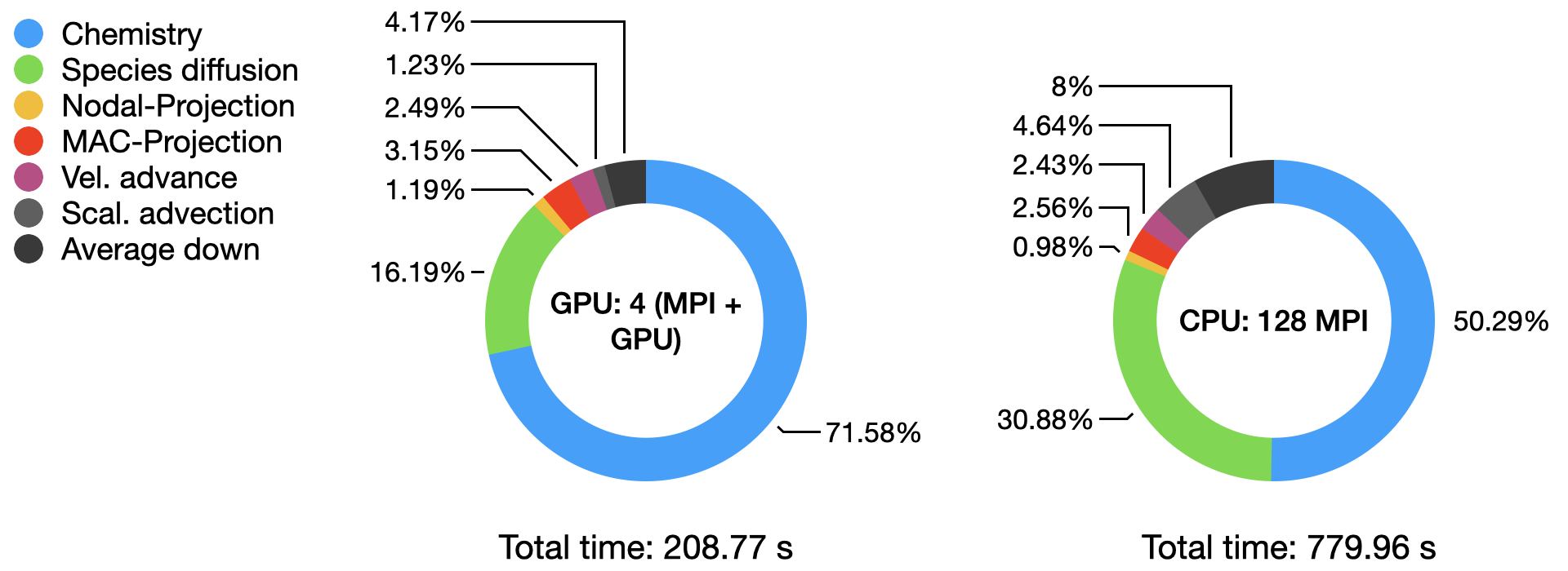
The total time comparison shows close to a 4x speed-up on a node basis on this platform, with the AMD Milan CPU being amongst the most performant to date. The detailed distribution of the computational time within each run highlight the dominant contribution of the stiff chemistry integration, especially on the GPU.
Results on Crusher (ORNL)
Crusher is the testbed for DOE’s first ExaScale platform Frontier. Crusher’s nodes consists of a single AMD EPYC 7A53 (Trento), 64 cores CPU connected to 4 AMD MI250X, each containing 2 Graphics Compute Dies (GCDs) for a total of 8 GCDs per node. When running with GPU acceleration, PeleLMeX will use 8 MPI ranks with each access to one GCD, while when running on flat MPI, we will use 64 MPI-ranks.
The FlameSheet case is ran using 2 levels of refinement (3 levels total) and the following domain size and cell count:
geometry.prob_lo     = 0.0 0.0 0.0        # x_lo y_lo (z_lo)
geometry.prob_hi     = 0.016 0.016 0.016  # x_hi y_hi (z_hi)

amr.n_cell           = 64 64 64
amr.max_level        = 2
leading to an initial cell count of 6.545 M, i.e. 0.8M/cells per GPU. The git hashes of PeleLMeX and its dependencies for these tests are:
================= Build infos =================
PeleLMeX    git hash: v22.12-15-g769168c-dirty
AMReX       git hash: 22.12-15-gff1cce552-dirty
PelePhysics git hash: v0.1-1054-gd6733fef
AMReX-Hydro git hash: cc9b82d
===============================================
The graph below compares the timings of the two runs obtained from AMReX TinyProfiler. Inclusive averaged data are presented here, for separates portion of the PeleLMeX algorithm (see the algorithm page for more details):
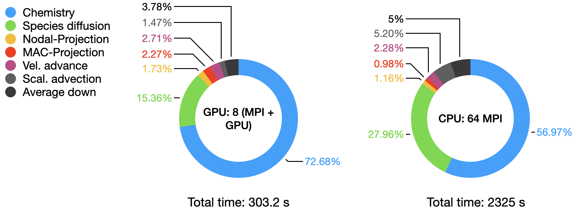
The total time comparison shows more than a 7.5x speed-up on a node basis on this platform, The detailed distribution of the computational time within each run highlight the dominant contribution of the stiff chemistry integration, especially on the GPU.
Results on Summit (ORNL)
Summit was launched in 2018 as the first DOE’s fully GPU-accelerated platform. Summit’s nodes consists of a two IBM Power9 CPU connected to 6 NVIDIA V100 GPUs. When running with GPU acceleration, PeleLMeX will use 6 MPI ranks with each access to one V100, while when running on flat MPI, we will use 42 MPI-ranks. Note that in contrast with newer GPUs available on Perlmutter or Crusher, Summit’s V100s only have 16GBs of memory which limit the number of cells/GPU. For this reason, the chemical linear solver used within Sundials is modified to the the less memory demanding cuSparse solver:
cvode.solve_type = sparse_direct
The FlameSheet case is ran using 2 levels of refinement (3 levels total) and the following domain size and cell count:
geometry.prob_lo     = 0.0 0.0 0.0        # x_lo y_lo (z_lo)
geometry.prob_hi     = 0.004 0.008 0.016  # x_hi y_hi (z_hi)

amr.n_cell           = 16 32 64
amr.max_level        = 2
leading to an initial cell count of 0.819 M, i.e. 0.136M/cells per GPU. The git hashes of PeleLMeX and its dependencies for these tests are:
================= Build infos =================
PeleLMeX    git hash: v22.12-15-g769168c-dirty
AMReX       git hash: 22.12-15-gff1cce552-dirty
PelePhysics git hash: v0.1-1054-gd6733fef
AMReX-Hydro git hash: cc9b82d
===============================================
The graph below compares the timings of the two runs obtained from AMReX TinyProfiler. Inclusive averaged data are presented here, for separates portion of the PeleLMeX algorithm (see the algorithm page for more details):
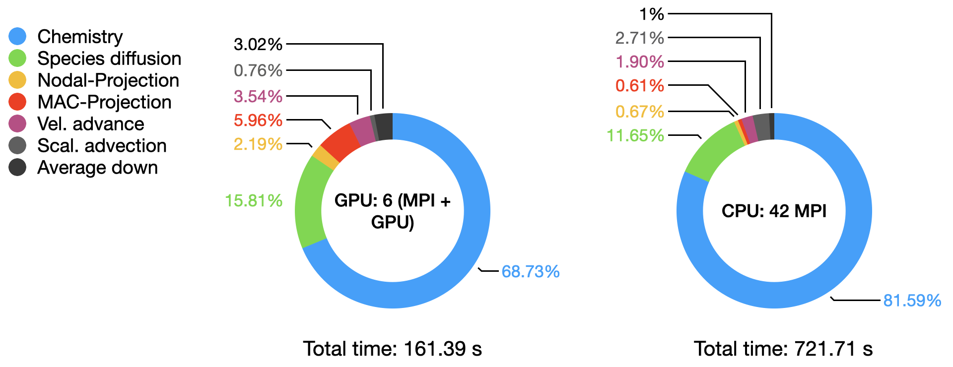
The total time comparison shows close to a 4.5x speed-up on a node basis on this platform, The detailed distribution of the computational time within each run highlight the dominant contribution of the stiff chemistry integration,
System comparison
It is interesting to compare the performances of each system on a node basis, normalizing by the number of cells to provide a node time / million of cells.
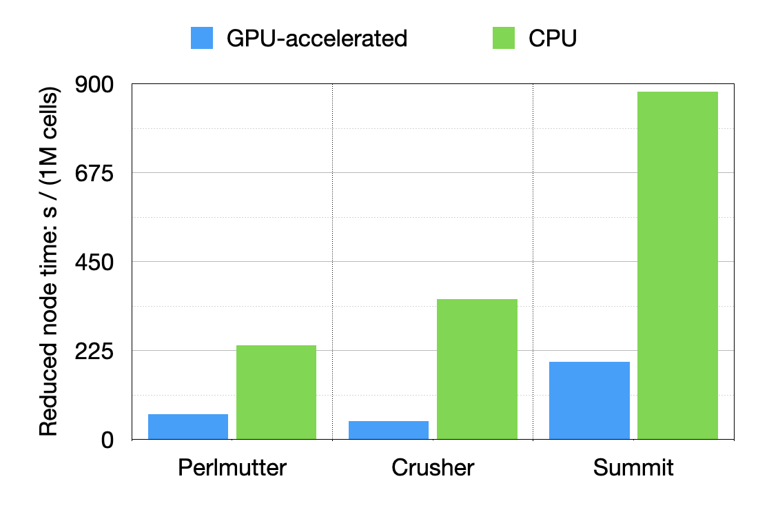
Results show that a 3x and 4.2x speed is obtained on a node basis going from Summit to more recent Perlmutter or Crusher, respectively.
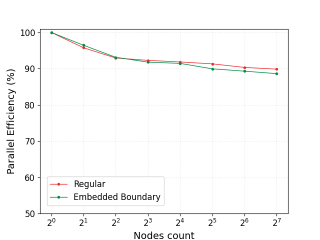
Weak scaling performances: FlameSheet case
Case description
Once again the case of a laminar premixed flame with harmonic perturbations is employed. On a single node, the case is similar to the one used in the previous section. To perform the weak scaling study (characterising the ability of the solver to scale up while keeping the same amount of work per compute unit), the dimensions of the computational domain are increased by a factor 2 in \(x\) and \(y\) alternatively as the number of compute nodes is doubled. The periodicity of the initial conditions allow to ensure that the amount of work per node remains constant.
To provide a more comprehensive test of PeleLMeX, the scaling study is also reproduced in the case of a flame freely propagating in a quiescient mixture towards an EB flat wall. The presence of the EB triggers numerous changes in the actual code path employed (from advection scheme to linear solvers).
The stude is performed on ORNL’s Crusher machine and the FlameSheet case is ran using 2 levels of refinement (3 levels total) and the following domain size and cell count:
geometry.prob_lo     = 0.0 0.0 0.0        # x_lo y_lo (z_lo)
geometry.prob_hi     = 0.016 0.016 0.016  # x_hi y_hi (z_hi)

amr.n_cell           = 64 64 64
amr.max_level        = 2
When introducing the EB plane, the following EB definition is employed:
eb2.geom_type     = plane
eb2.plane_point   = 0.00 0.00 0.0004
eb2.plane_normal  = 0 0 -1.0
and because nothing interesting is happening at the EB surface, it is maintained on the base level using the following parameters:
peleLM.refine_EB_type = Static
peleLM.refine_EB_max_level = 0
peleLM.refine_EB_buffer = 2.0
The parallel efficiency, defined as the time to solution obtained on a single node divided by the time to solution obtained with an increasing number of nodes is reported in the figure below for the case wo. EB and w. EB. The efficiency is found to drop to 90% when going from 1 to 128 Crusher nodes (8 to 1024 GPUs) and a closer look at the scaling data shows that most of the efficiency loss is associated with the communication intensive linear solves.