PeleLMeX Verification & Validations
This section assembles results of PeleLMeX simulations on a set a test cases for which a reference solution can be obtained from the literature or an analytical solution exists.
Laminar premixed flame
The case of a laminar premixed flame is a foundational test case for a reactive
flow solver. A laminar premixed flame setup is available in Exec/RegTests/FlameSheet.
The case reported hereafter is that of a planar laminar methane/air flame at
atmospheric conditions and a lean equivalence ratio of 0.9. The initial condition
is obtained from a Cantera simulation using
the DRM19 mechanism and the simulation is conducted starting with a coarse resolution
\(d_{l,0}/\delta_x = 3.5\) (3.5 grid cells in the flame thermal thickness) and progressively
refined to \(d_{l,0}/\delta_x = 110\) using AMR. Note that the simulation is carried for
about 30 \(\tau_f = d_{l,0} / S_{l,0}\) before adding refinement levels ensuring that initial
numerical noise introduced by interpolating the Cantera solution onto the cartesian grid is
completely removed.
The PeleLMeX results obtained with the finest grid are compared to that of Cantera in Fig. 3. Profiles of major and intermediate species as well as temperature across the flame front are displayed, with Cantera results shown as black ticked lined underlying each continuous line obtained with PeleLMeX, demonstrating the solver accuracy.
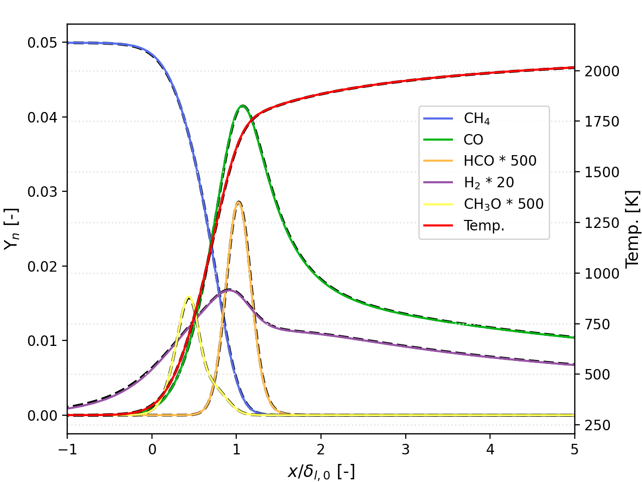
Fig. 3 : One-dimentional flame profiles with PeleLMeX and Cantera (underlying black dashed lines)
It is interesting to see how resolution affect the prediction of PeleLMeX. The Table 1 shows the laminar flame speed, obtained by numerically integrating the fuel consumption rate, at increasing level of refinement. For each AMR level addition, simulation are conducted for about 10 \(\tau_f\), until the flame speed stabilizes. With only a handful of cells across the flame thermal thickness, the flame speed is recovered with an accuracy close to 1.5%.
\(d_{l,0}/\delta_x\) [-] |
3.44 |
6.88 |
13.8 |
27.5 |
55 |
110 |
|---|---|---|---|---|---|---|
\(S_{l,0}\) [m/s] |
0.35696 |
0.35144 |
0.35408 |
0.35473 |
0.35488 |
0.35494 |
Error (vs. Cantera) [%] |
0.02 |
1.54 |
0.8 |
0.6 |
0.58 |
0.57 |
Additionally, Fig. 4 compares profiles of major and intermediate species as well as temperature across the flame front for the coarsest and the finest resolution employed. Results indicates that major species (or temperature) are well captured whereas short lived species peak values are locally off due to the lack of resolution but are still reasonably well located within the flame front.
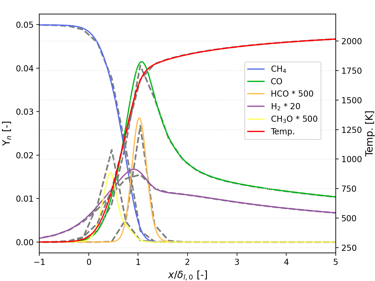
Fig. 4 : Comparison of a coarsed and finely resolved 1D flame in PeleLMeX
Laminar Poiseuille flow
The laminar pipe flow or Poiseuille flow, is a basic test case for wall bounded flows. In the present configuration, the geometry consist of a circular channel of radius \(R\) = 1 cm aligned with the \(x\)-direction, where no-slip boundary conditions are imposed on EB surface. The flow is periodic in the \(x\)-direction and a background pressure gradient \(dp /dx\) is used to drive the flow.
The exact solution at steady state is:
where \(G = -dp/dx\), and \(\mu\) is the dynamic viscosity.
The test case can be found in Exec/RegTests/EB_PipeFlow, where
the input parameters are very similar to the PeleC counterpart of
this case.
The steady-state \(x\)-velocity profiles across the pipe diameter at increasing resolution are plotted along with the theorerical profile in Fig. 5:
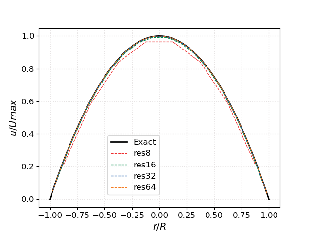
Fig. 5 : Axial velocity profile at increasing resolution with PeleLMeX
A more quantitative evaluation of PeleLMeX results is obtained by calculating the L2 norm of the error against the analytical profile:
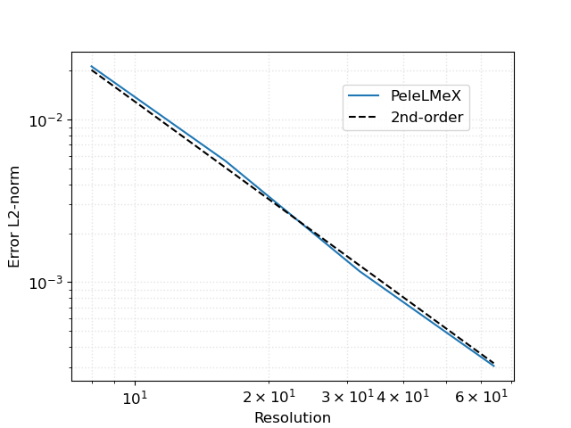
Fig. 6 : L2-norm of the axial velocity profile as function of the number of cells across the pipe diameter
showing second-order convergence for this diffusion dominated flow.
Taylor-Green vortex breakdown
The Taylor-Green vortex breakdown case is a classical CFD test case described in here (case C3.3). It is intended to test the capability of the code to capture turbulence accurately, with the flow transitioning to turbulence, with the creation of small scales, followed by a decay phase similar to decaying homogeneous turbulence.
Building and running
The test case can be found in Exec/RegTests/TaylorGreen.
$ make -j 16 DIM=3 USE_MPI=TRUE TPL
$ make -j 16 DIM=3 USE_MPI=TRUE
$ mpiexec -n 16 $EXECUTABLE inputs_3d amr.ncell=64 64 64
The user can run a convergence study by varying amr.ncell.
Results
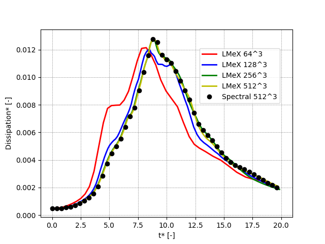
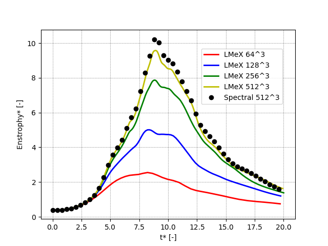
The following figures shows the kinetic energy, the dissipation rate and the enstrophy as function of time (all quantities are non-dimensional) for increasing resolutions (ranging from 64^3 to 512^3) and compared to the results of a high-order spectral solver with a 512^3 resolution. PeleLMeX results are obtained with the Godunov_PPM scheme and show that even though PeleLMeX uses a 2nd-order scheme, reasonable accuracy compared to the spectral results is obtained when the resolution is sufficient.

Additionally, it is interesting to compare the different advection schemes available in PeleLMeX (namely, Godunov_PLM, Godunov_PPM, Godunov_BDS, Godunov_PPM_WENOZ) at a fixed 256^3 spatial resolution:
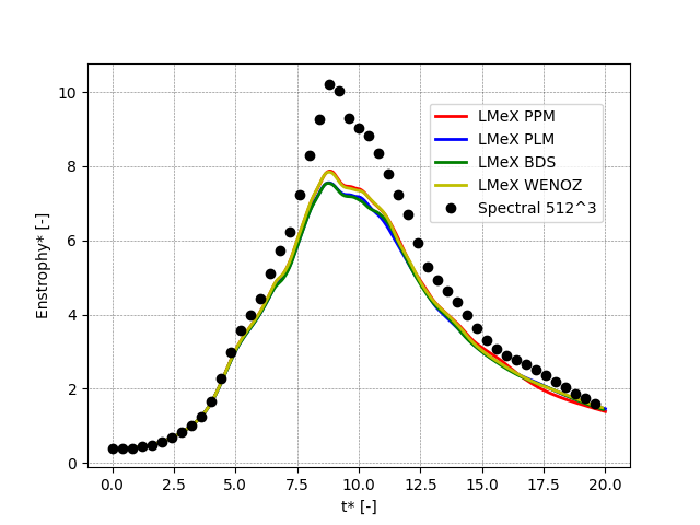
On this particular case, the differences between the advection schemes are fairly marginal compared to those observed at different grid resolutions.
Channel Flow using EB
We present results of the classical periodic channel flow, available in the
Exec/RegTests/EB_PipeFlow folder. Simulations are performed at three
stress Reynold number \(Re_{\tau}\) = 180, 395 and 934 corresponding
to the cases described in Kim et al., 1986,
Moser et al., 1999 and
Hoyas and Jimenez, 2006, respectively. A first
DNS is performed at \(Re_{\tau}\) = 180, then the LES models implementation is tested
at higher Reynold numbers.
For all cases, the configuration is periodic in the \(x\) and \(z\) directions and wall boundaries are imposed in the \(y\) direction using Embedded Boundaries.
DNS results at \(Re_{\tau}\) = 180
The channel half width \(\delta\) is set to 0.005 m, and the computational domain extend in +/- 0.0052 m in \(y\) with EB intersecting the domain at +/- \(\delta\). A background pressure gradient in imposed in the \(x\) to compensate wall friction. The base grid and two levels of refinement are described in Table 2:
\(x\) |
\(y\) |
\(z\) |
|
|---|---|---|---|
Domain size |
6.24 \(\delta\) |
2.08 \(\delta\) |
3.12 \(\delta\) |
Base grid L0 |
384 |
128 |
192 |
L1 |
768 |
256 |
384 |
L2 |
1536 |
512 |
768 |
The fluid in the simulation is air at ambient pressure and a temperature of 750.0 K, the physical property of which are summarized in Table 3:
Pressure |
Temperature |
Density |
\(\mu\) |
\(\nu\) |
|
|---|---|---|---|---|---|
Value [MKS] |
102325.0 |
750.0 |
0.468793 |
3.57816e-5 |
7.63271e-5 |
The characteristics of the flows are reported in Table 4:
\(Re_{\tau}\) |
\(u_{\tau}\) |
\(\tau_w\) |
\(dp/dx\) |
\(t^* = \delta/u_{\tau}\) |
|---|---|---|---|---|
180.2 |
2.75122 |
3.5485 |
-709.79 |
1.817e-3 |
Two levels of refinement, targeted on the EB, are employed in order to sufficiently resolve the boundary layer. The mesh characteristics are summarized in Table 5. The \(y^+\) value is that of the cell center of the first full cell (uncut by the EB).
\(Re_{\tau}\) |
\(\Delta y^+ L0\) |
\(\Delta y^+ Lmax\) |
\(y^+\) |
Cells count |
|---|---|---|---|---|
180.2 |
2.93 |
0.732 |
0.479 |
56.6 M |
Simulations are carried out for 20 eddy turn over time \(t^*\) to reach statistically steady conditions and data are then spatially averaged in the periodic directions and averaged in time over 10 \(t^*\) to get the velocity statistics in the direction normal to the wall.
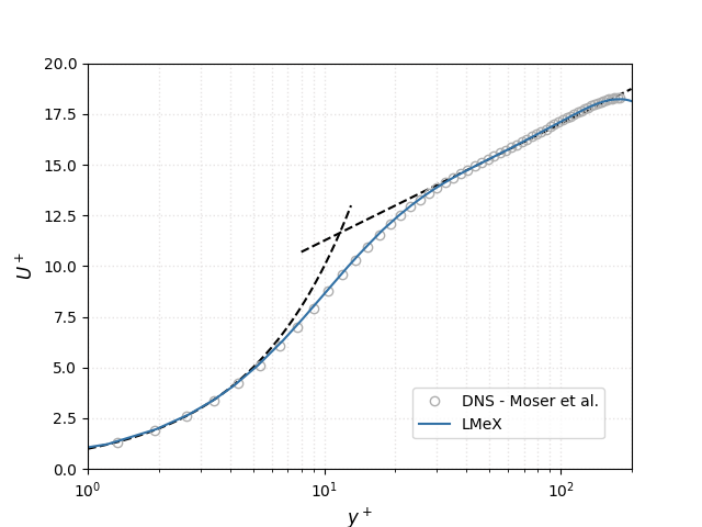

Results indicate that PeleLMeX is able to reproduce accurately the DNS data obtained with a high-order spectral solver, provided sufficient resolution at the wall.
LES results at \(Re_{\tau}\) = 395, 934
The channel half width \(\delta\) is set to 0.01 m, and the computational domain extend in +/- 0.0101 m in \(y\) with EB intersecting the domain at +/- \(\delta\). The base grid is coarser than the DNS one by a factor of 2. A background pressure gradient in imposed in the \(x\) to compensate wall friction. The fluid conditions are similar to that of the DNS case and the flow and mesh characteristics are summarized in Table 6:
\(Re_{\tau}\) |
\(u_{\tau}\) |
\(\tau_w\) |
\(dp/dx\) |
\(t^* = \delta/u_{\tau}\) |
\(\Delta y^+ L0\) |
\(\Delta y^+ Lmax\) |
|---|---|---|---|---|---|---|
395 |
3.01492 |
4.26121 |
-426.121 |
3.3317e-3 |
12.467 |
6.2336 |
934 |
7.12895 |
23.8250 |
-2382.50 |
1.4027e-3 |
29.479 |
7.36984 |
Note that a single level of refinement is employed for the \(Re_{\tau}\) = 395 while two are used for \(Re_{\tau}\) = 934 in order to provide sufficient (but still below \(y^+=1\)) resolution near the walls.
Simulations are performed with the WALE LES SGS model. The plots below shows that PeleLMeX is able to reproduce the normalized velocity profile reasonably well even though the resolution requirements for a Wall Resolved LES are not quite attained with the grid employed here.
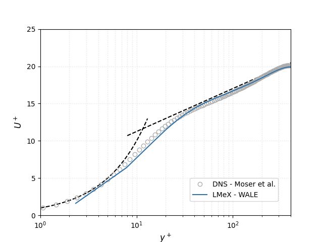


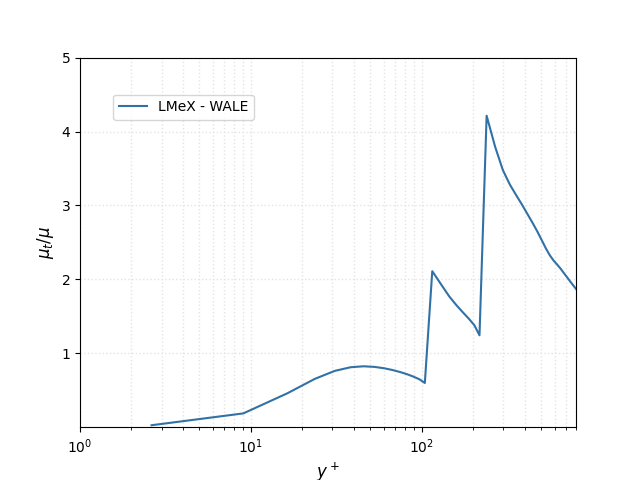
The velocity variance in the plot above show distinctive drops around coarse/fine interfaces, where the filter size change and a the subgrid-scale contribution increases as depicted on the figure below showing the subgrid-scale viscosity for the \(Re_{\tau}\) = 934 case.
Further work is ongoing to assess how to better handle large LES filter size changes in the context of AMR-LES
Laminar counterflow diffusion flame
The laminar counterflow diffusion flame is a fundamental test case for non-premixed reactive flows. A
laminar counterflow diffusion flame setup is available in Exec/Production/CounterFlow.
In the present configuration, the geometry consists of a 1.5 cm x 1.5 cm domain with inflow at the left
and right boundaries and outflow at the top and bottom boundaries. The left and right inflow boundaries
correspond to the oxidizer and fuel inlet sides respectively, with an oxidizer/fuel jet section of
diameter \(d_{jet} = 0.5 cm\) (prob.jet_radius of 0.0025) centered at the boundary. The
remainder of the inflow boundary consists of inert inflow sections with composition of pure N2.
The oxidizer jet section composition is that of air, while the fuel jet section composition is pure
gaseous Dodecane. The inert inflow velocity on the left and right is set equal to the oxidizer and fuel
jet velocities, respectively, in order to eliminate shear interactions between the inert and jet
streams. The oxidizer and fuel jet velocities are 15.0 cm/s and 6.17 cm/s, respectively, corresponding
to a global strain rate of \(40 s^{-1}\). The initial condition corresponds to air composition
filling the left half of the domain and gaseous Dodecane composition filling the right half of the
domain with a hyperbolic tangent smoothly transitioning species mass fractions in the center of the
domain. Ignition is performed by patching a spherical kernel of elevated temperature (in this case
1000 K) with radius of 0.3 cm in the center of the domain as to cause autoignition. Grid refinement
criteria based on the gradient of temperature is used and solution convergence is achieved with
amr.max_level of 2.
The PeleLMeX results obtained using the specified grid refinement criteria are compared to that of Cantera in spatial and mixture fraction space in Fig. 7 and Fig. 8, respectively. Centerline profiles of major species as well as temperature across the flame front at steady-state are displayed, with PeleLMeX results indicated by solid colored lines and Cantera results indicated by black ticked lines. The results show very good agreement between the PeleLMeX and Cantera centerline profiles, with only small differences visible when plotting versus spatial coordinate due to differences in geometry (1-D vs. 2-D).
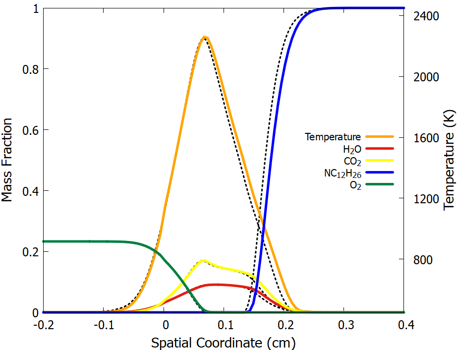
Fig. 7 : One-dimentional flame spatial profiles with PeleLMeX and Cantera (underlying black dashed lines)
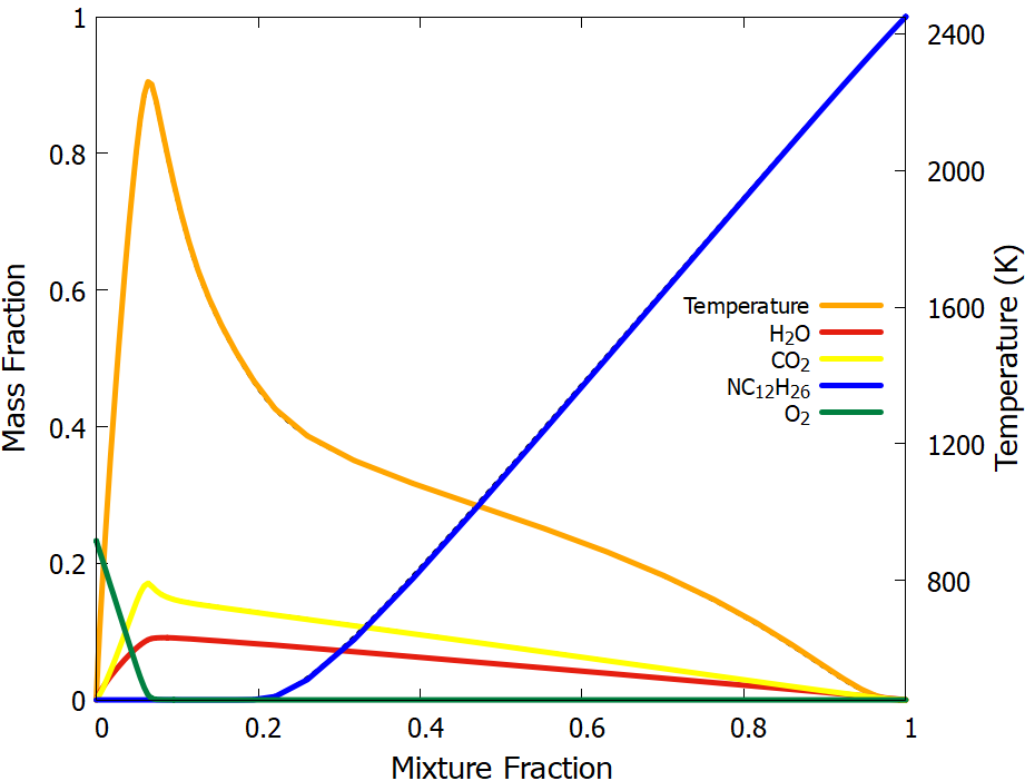
Fig. 8 : One-dimentional flame profiles (mixture fraction space) with PeleLMeX and Cantera (underlying black dashed lines)