Analytically reduced chemistry via quasi-steady state (QSS) assumption in PelePhysics
The QSS assumption
Given a detailed chemical mechanism, some species can sometimes be assumed to be in a quasi-steady state (QSS). Formally, if species \(A\) is assumed to be in a QSS then
where \([A]\) is the molar concentration of species \(A\). If the set of QSS species is judiciously chosen, macroscopic quantities of interest such as ignition delay or laminar flame speed are only mildly affected by the QSS assumption [DRG2005].
The advantage of the QSS assumption
Using the elementary reactions of the chemical mechanism, it is possible to write a set of algebraic equations that relate QSS species to non-QSS species. In turn, it is not necessary to transport the QSS species in the flow solver, as their concentration can be directly obtained from the non-QSS species.
In addition, QSS species are typically species that induce stiffness in the chemical mechanism since they evolve on scales different that the non-QSS species.
From non-QSS species to QSS species concentration
The set of algebraic equations that result from the QSS assumption does not always easily result in a simple algebraic relation between a given QSS species and all the non-QSS species. To do this, it is necessary to apply some form of linearization to the reactions involved [SYS2006]. In addition, even in the presence of linear relations, QSS species may depend on one another. The following figure shows the relation graph between the QSS species of a reduced \(N-C_{12}H_{26}\) mechanism [ND2018]. The arrows indicate that a QSS species concentration depends on another QSS species concentration. It can also be seen that dependency groups exist among the QSS species. In PelePhysics it is possible to deduce invert analytically the linear system of equations given an arbitrary relation graph.
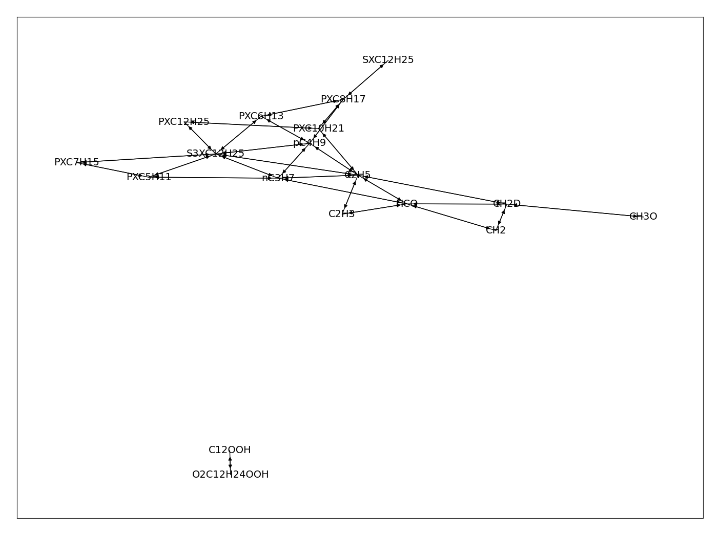
4 Relation graph between QSS species for N-dodecane mechanism [ND2018]
Linearizing the set of equations
In general, the QSS assumption results in a set of equations that are non-linearly coupled making it difficult to invert the system. The non-linear relations can arise if two or more QSS-species are on the same side of an elementary reaction, or if the stoichiometric coefficient of a QSS-species is not equal to one. Below, the relation graph between the QSS species plotted above is expanded with dots that denote reactions that relate QSS-species. Dots or species are colored in red if they are involved in a quadratic coupling.
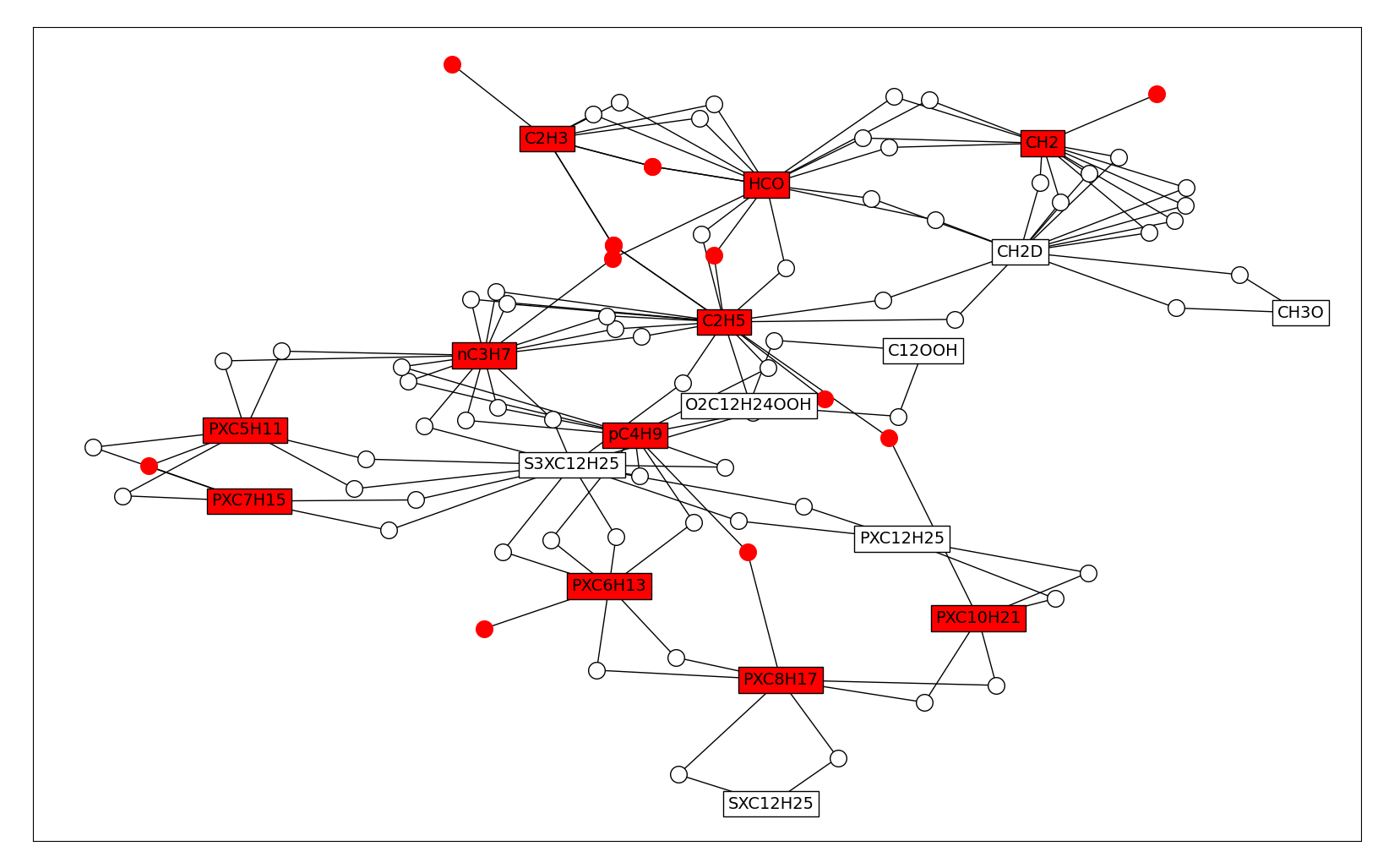
5 Graph of dependencies between QSS species for N-dodecane mechanism [ND2018], augmented with reactions. Red species or dots denote species and reactions involved in quadratic coupling.
From here, it is necessary to eliminate the quadratic coupling to linearize the set of algebraic equations that result from the QSS assumption. Three methods can be envisioned: either one relaxes the QSS assumption by reducing the set of QSS species (Method 1) or one can eliminate the reactions that induce quadratic coupling. In case reactions are reversible, it can happen that either the forward or the backward reaction induces the quadratic coupling. Either one can remove both the forward and the backward reaction (Method 2) or remove either the backward or the forward reaction (Method 3).
All three methods are available in PelePhysics. By default, Method 3 is activated as it is computationally efficient and accurate (as will be shown below). Method 1 is the most accurate and Method 2 is the most computationally efficient in our experience. Given that each method has its advantage, we decided to allow the user to choose either one according to his/her needs.
Validation
The three linearization methods are validated against the skeletal \(N-C_{12}H_{26}\) [SKEL2017]. Using 343 0D calculation that span the range of applicability of the QSS assumption (\(\phi = [0.5, 2.0], p=[1atm, 50atm], T=[800K, 1600K]\)), the ignition delay is computed using the skeletal mechanism (SK53) and each one of the three linearization methods for the QSS mechanism (RedXX). The left plot shows the correlation between the ignition delay from the skeletal mechanism and the reduced version. The statistics of the relative error between the reduced and the skeletal mechanism are shown in the title of that plot. The right plot shows the ignition delay values at high-pressure conditions only.
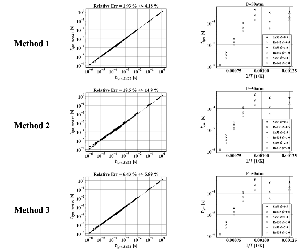
6 Left: Scatter plot of the ignition delay measured with the QSS mechanism linearized and the skeletal mechanism. Right: Ignition delays measured for the skeletal mechanism and QSS mechanism linearized at high-pressure conditions. Top: Method 1. Middle: Method 2. Bottom: Method 3.
Analytical Jacobian
In several computational experiments, using analytical Jacobians was found to provide better stability or efficiency compared with finite difference approximation or numerical inversion (see also fig:qss_integrator). Compared with non-QSS mechanisms, analytical Jacobians need to reflect the dependence of each QSS species on non-QSS species. However, QSS species may depend on an ensemble of other non-QSS species and therefore ensemble of reactions. Therefore, analytical Jacobian cannot be constructed by sequentially adding the contribution of each reaction. This significantly complicates the analytical jacobian generation. Failure to include the dependence of QSS species with respect to non-QSS species typically results in wrong ignition profiles, unless very small timesteps are used, as seen in figure fig:qss_aj.
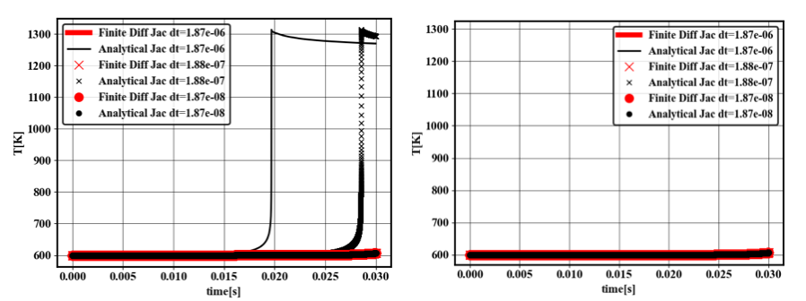
7 Temperature of a 0D reactor at constant pressure for NC12H26. Initial temperature is 600K, initial molar fraction of O2 is 0.7 and initial molar fraction of fuel is 0.3. Left: Results without inclusion of dependence of QSS species with respect to non-QSS species. Right: Result with inclusion of dependence of QSS species with respect to non-QSS species.
To ease the implementation of analytical Jacobian in presence of QSS species, a symbolic approach is used to construct the analytical Jacobian. This strategy has the advantage of not requiring complex logic, and being flexible and readable for future development. For the last row of the Jacobian (partial difference of reaction rate with respect to temperature), finite difference is used since perturbations in temperature are less susceptible to numerical errors than perturbations in species concentrations. During the construction of the reaction rates, the operations printed to file are recorded symbolically using the sympy and symengine library [SYMPY]. For computational efficiency during the symbolic differentiation, the chain-rules terms are computed and the final expressions are computed and assembled by chain-ruling using logic internal to CEPTR rather than sympy. We have found that this speeds up the Jacobian construction cost by a factor 10.
To activate the use of symbolic jacobian, one needs to pass the flag --qss_symbolic_jacobian to CEPTR.
Printing the Jacobian terms one by one is not possible since the expressions that include QSS species are typically very large. Instead, the expressions are reduced via common sub-expression precomputing that are later used in each term of the Jacobian. The number of subexpressions may be orders of magnitude larger than the number of Jacobian entries which can be problematic if the computational architecture has limited memory.
Several formatting strategies have been implemented to mitigate the memory footprint of the symbolic Jacobian. They can be adjusted by providing a .toml file to CEPTR via the qss_format_input flag. A model input file is provided in the Tutorials section of this documentation. A model execution script for generating a mechanism for dodecane_lu_qss is available under the Tutorials section of this documentation.
The formatting options are the following
hformat(string)cpuwill print intermediate variables used for chainruling. This gives a “readable” version of the Jacobian entries, albeit memory consuming.gpuwill not print intermediate variables used for chainruling, and instead will replace them directly in the Jacobian entries. This gives a less readable version of the Jacobian, but more memory efficient.
remove_1(boolean) will replace expressions of the type1.0 * xxxintoxxx.remove_pow(boolean) will convert expressions of the typepow(xxx,n)into multiplications or division. The conversion occurs forn<=3andn>=-3consistent with optimCudaremove_pow10(boolean) will convert expressions of the typepow(10,xxx)intoexp(ln(10)*xxx), consistent with optimCudamin_op_count(integer) counts number operations used to construct each common subexpression and replace the common subexpression if the number of operations is less or equal tonmin_op_count_all(integer) is similar tomin_op_countbut also counts how many times that common subexpression is used later. The meaning ofnis different than formin_op_countas it refers to how many more operations will be done if the common subexpression is eliminated. This option should be preferred tomin_op_countas it tends to only marginally increase the file size (therefore compile time), while still being memory efficient.gradual_op_count(boolean) is useful ifmin_op_countormin_op_count_allare active. It loops from 1 tonand gradually eliminate the common subexpressions. This has the advantage of ensuring that the memory footprint is strictly monotonically decreasing as n is increased.store_in_jacobian(boolean) will use the Jacobian array as a temporary space to store intermediate variables. In particular, the last row of the Jacobian (dependence with respect to temperature) is done by finite difference which requires storing intermediate variables (production rate, forward and backward reactions). When the option is active, theproductionRatefunction used to compute the finite difference is replaced with aproductionRate_lightfunctions where references to different parts of the Jacobian are used in place of allocating new arrays.round_decimals(boolean) will round floats printed bysympywhen possible to minimize character count in themechanism.Hfile.recycle_cse(boolean) will reuse subexpressions that are not used later to avoid declaring new temporary reals.remove_single_symbols_cse(boolean) will remove common subexpressions that are made of 1 operation and 1 symbol. Those common subexpressions are typically-xxxand may not appear as worth replacing because they save 1 operations and are reused multiple times. However, when replaced in the later expressions, the-operations typically disappear or is merged into another operations which actually does not increase the total number of operations.
The analytical Jacobian for QSS mechanisms is typically more accurate and stable than GMRES, and is on par with the finite difference Jacobian of CVODE as seen in fig:qss_integrator
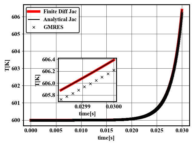
8 Temperature of a 0D reactor at constant pressure for NC12H26. Initial temperature is 600K, initial molar fraction of O2 is 0.7 and initial molar fraction of fuel is 0.3. Results are shown for finite difference jacobian (red thick line), analytical jacobian (black line) and GMRES (crosses) using the same tolerances.
In terms of speed, the analytical Jacobian 0D reactor is faster on CPU than finite difference Jacobian and GMRES. For the piston bowl challenge problem, the analytical Jacobian relative speed depends on the prevalence of chemical reactions. At some points, the AJ is slower than GMRES with PeleC, at others, AJ is faster. In PeleLM cases, AJ was found to be faster than GMRES. Further optimization and tests are still ongoing.
Using the Analytical Jacobian
To use the analytic Jacobian QSS mechanisms in a Pele run, one must specify the correct solve_type. The choice of the solve_type will determine whether or not the analytic Jacobian is used. With CUDA, both magma_direct and sparse_direct will use the analytic Jacobian, while on HIP only magma_direct will trigger the use of the analytic Jacobian parts.
Lu, C. K. Law, A directed relation graph method for mechanism reduction, Proceedings of the combustion institute, 30(1):1333-1341, 2005.
Lu, C. K. Law, Systematic approach to obtain analytic solutions of quasi steady state species in reduced mechanisms, The Journal of Physical Chemistry A, 110(49):13202-13208, 2006.
Borghesi, A. Krisman, T. Lu, J. H. Chen, Direct numerical simulation of a temporally evolving air/n-dodecane jet at low-temperature diesel-relevant conditions, 195:183-202, 2018.
Yao, Y. Pei, B. J. Zhong, S. Som, T. Lu, K. H. Luo, A compact skeletal mechanism for n-dodecane with optimized semi-global ! low-temperature chemistry for diesel engine simulations, 191:339-349, 2017.
Meurer, C. P. Smith, M. Paprocki, O. v{C}ert'{i}k, S. B. Kirpichev, M. Rocklin, A. Kumar, S. Ivanov, J. K. Moore, S. Singh, T. Rathnayake, S. Vig, B. E. Granger, R. P. Muller, F. Bonazzi, H. Gupta, S. Vats, F. Johansson, F. Pedregosa, M. J. Curry, A. R. Terrel, S. Rouv{c}ka, A. Saboo, I. Fernando, S. Kulal, R. Cimrman, A. Scopatz, SymPy: symbolic computing in Python, 3:e103, 2017.