Validation of PeleC
The PeleC validation plan is aimed at exercising and validating the PeleC reacting flow capabilities. The following cases, described further on, are used for validation.
Decay of homogeneous isotropic turbulence
Non reacting Taylor-Green vortex breakdown
Reacting Taylor-Green vortex breakdown
Counter flow diffusion flame
Counter flow premixed flame
Flame-Vortex interaction
Sandia Flame D
Premixed ignition kernel in isotropic turbulence
Warning
This section is a work in progress. Several of these cases have yet to be performed and are noted as such.
Decay of homogeneous isotropic turbulence
Simulations were performed for turbulent Mach number = 0.1, Taylor scale based Reynolds number = 100, Prandtl number = 0.71, and k0 = 4 at several different resolutions (uniform discretization, no AMR) using a prescribed energy spectrum.
The definitions for the different quantities and reference data (in black) can be found in Johnsen et al. (2009) JCP and Movahed and Johnsen (2015) JFM. VisIt was used to post-process some quantities using visit_pp_aux_vars.py (located in the Exec/HIT folder) with the command
$ visit -nowin -cli -s Exec/RegTests/visit_pp_aux_vars.py
Generating the initial conditions
The initial conditions for this validation problem are derived from the following energy spectrum:
and can be generated with the Python script in the PelePhysics TurbFileHIT support code.
Building and running
The decay of homogeneous isotropic turbulence case can be found in Exec/RegTests/HIT:
$ make -j 16 DIM=3 USE_MPI=TRUE
$ mpiexec -n 36 $EXECUTABLE inputs_3d
The user can run a convergence study by generating initial conditions
for higher resolutions and varying amr.ncell.
Results
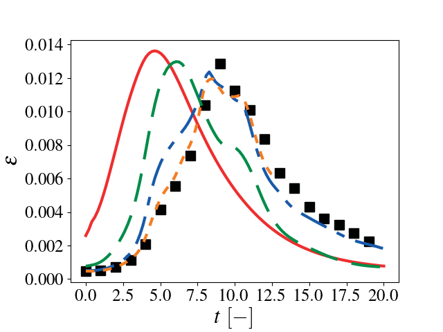
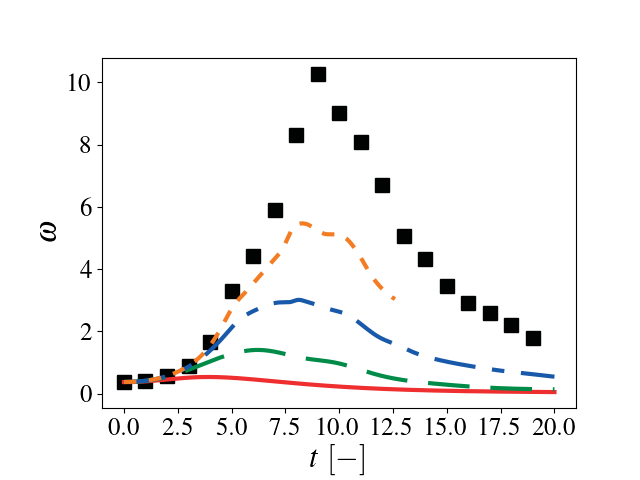
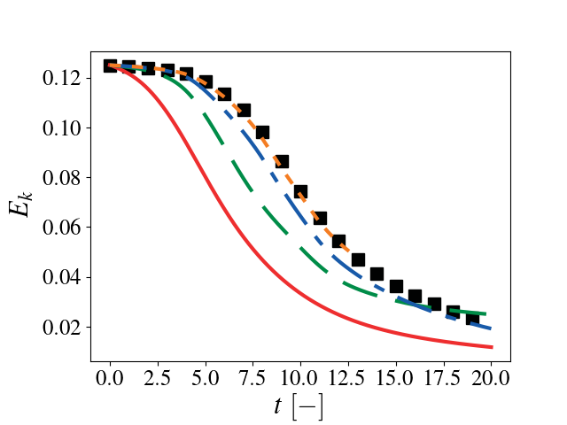
As the resolution increases, there is good agreement between the Pele data and reference data.
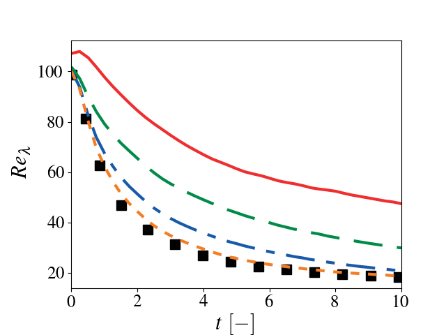
11 Reynolds number as a function of time. Solid red: \(32^3\), dashed green \(64^3\), dash-dotted blue: \(128^3\), dotted orange: \(256^3\), black squares: Johnsen et al. (2009) JCP.
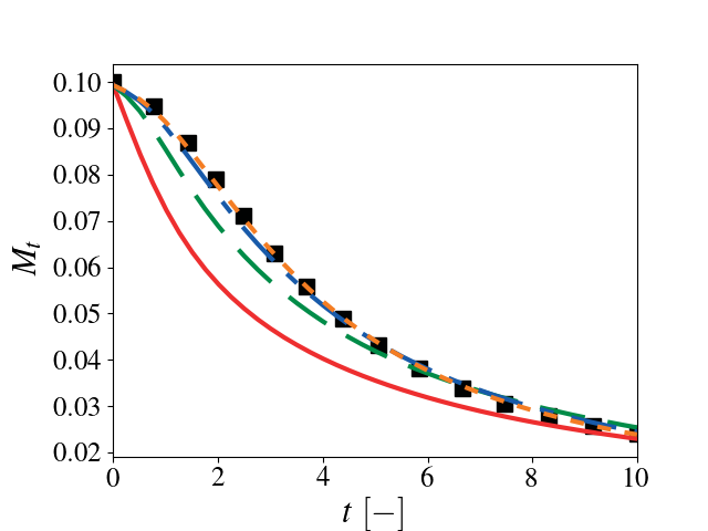
12 Mach number as a function of time. Solid red: \(32^3\), dashed green \(64^3\), dash-dotted blue: \(128^3\), dotted orange: \(256^3\), black squares: Johnsen et al. (2009) JCP.
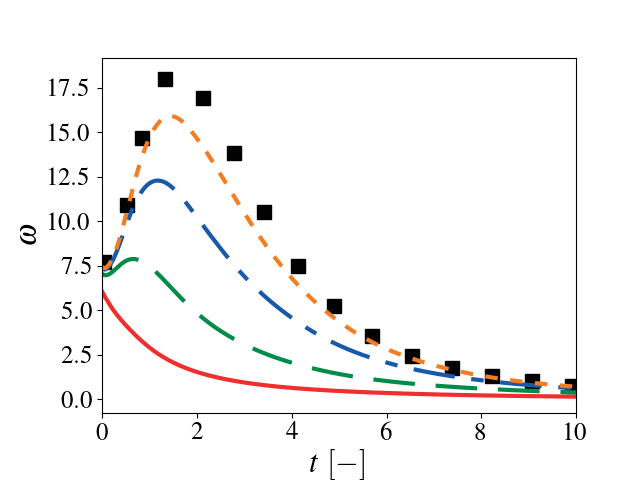
13 Enstrophy as a function of time. Solid red: \(32^3\), dashed green \(64^3\), dash-dotted blue: \(128^3\), dotted orange: \(256^3\), black squares: Johnsen et al. (2009) JCP.
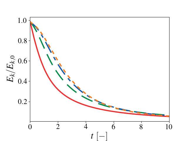
14 Kinetic energy as a function of time. Solid red: \(32^3\), dashed green \(64^3\), dash-dotted blue: \(128^3\), dotted orange: \(256^3\).
Taylor-Green vortex breakdown
This setup is one of the test problems outlined by the High-Order CFD workshop. A complete description of the problem can be found at NASA HOCFDW website and the reference data is found here. More details of the problem and methods used to obtain the reference data can be found in Bull and Jameson (2014) 7th AIAA Theoretical Fluid Mechanics Conference (doi: 10.2514/6.2014-3210) and DeBonis (2013) 51st AIAA Aerospace Sciences Meeting (doi:10.2514/6.2013-382).
Building and running
The Taylor-Green vortex breakdown case can be found in Exec/RegTests/TG:
$ make -j 16 DIM=3 USE_MPI=TRUE
$ mpiexec -n 36 $EXECUTABLE inputs_3d amr.ncell=64 64 64
The user can run a convergence study by varying amr.ncell.
Results
As the resolution increases, there is good agreement between the Pele data and reference data.
15 Dissipation as a function of time. Solid red: \(32^3\), dashed green \(64^3\), dash-dotted blue: \(128^3\), dotted orange: \(256^3\), black squares: HOCFDW.
16 Enstrophy as a function of time. Solid red: \(32^3\), dashed green \(64^3\), dash-dotted blue: \(128^3\), dotted orange: \(256^3\), black squares: HOCFDW.
17 Kinetic energy as a function of time. Solid red: \(32^3\), dashed green \(64^3\), dash-dotted blue: \(128^3\), dotted orange: \(256^3\), black: HOCFDW.
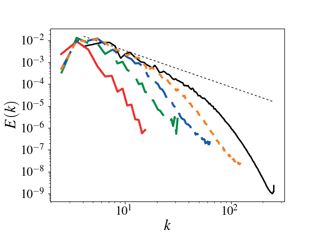
18 Spectrum at \(t=9 t_c\). Solid red: \(32^3\), dashed green \(64^3\), dash-dotted blue: \(128^3\), dotted orange: \(256^3\), black: HOCFDW.
Reacting Taylor-Green vortex breakdown
This test case is based on work by Abdelsamie et al. (Mini-Symposium on Verification and Validation of Combustion DNS, 17th Int. Conference on Numerical Combustion, Aachen, Germany May 7, 2019 where a Taylor-Green vortex setup used in non-reacting CFD is adapted to a reacting flow configuration. Comparison of results from several well-established codes such as Nek5000, DINO and YALES are provided in the workshop documentation. We have performed the entire suite of cases described in the workshop documentation and only present the final 3D reacting case.
Good comparisons with the reference simulations were obtained in most of the quantities of interest.
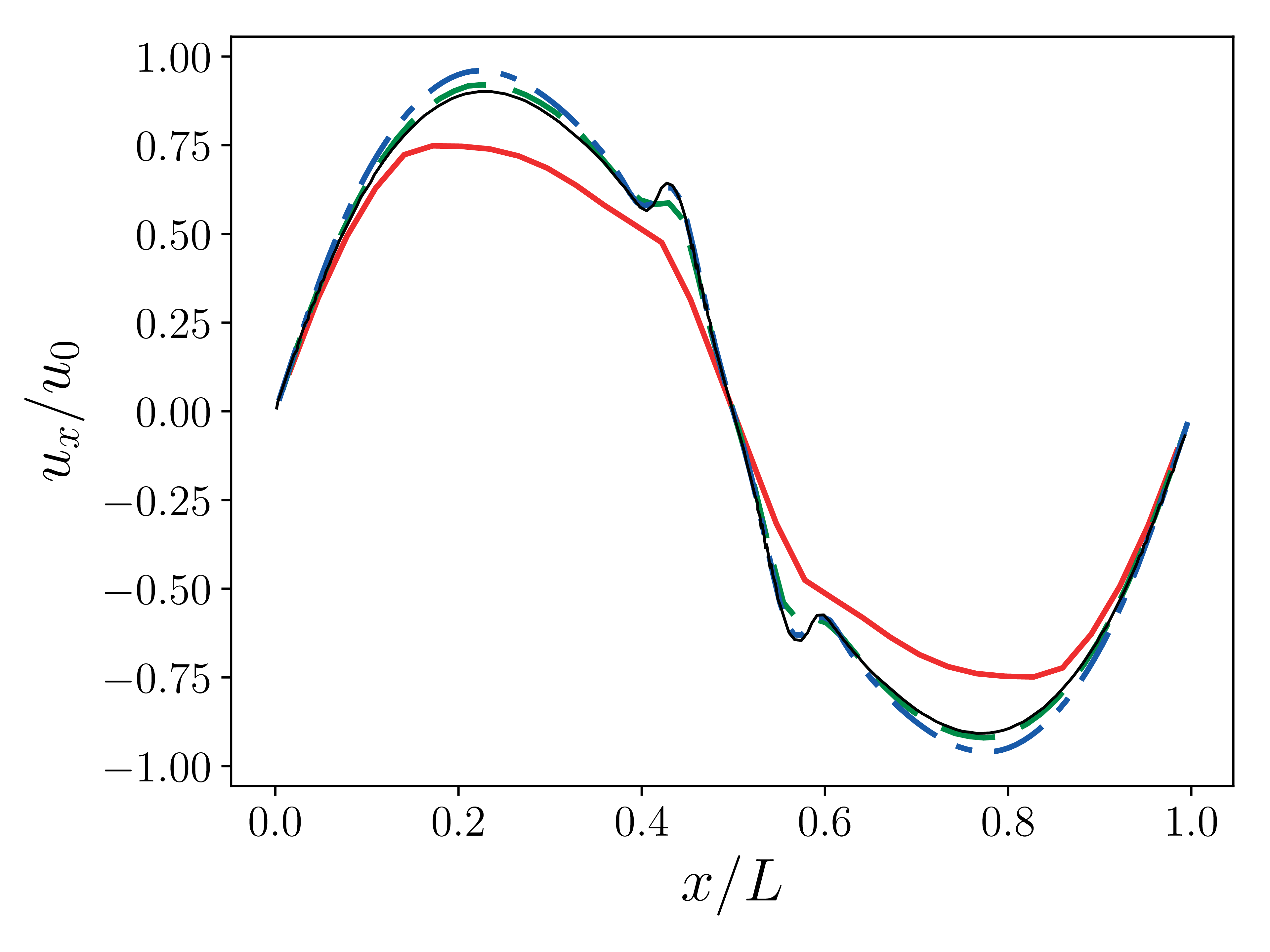
19 \(x\)-velocity at \(t=5e-4 \tau\). Solid red: \(32^3\), dashed green \(64^3\), dash-dotted blue: \(128^3\), black: reference solution (DINO).
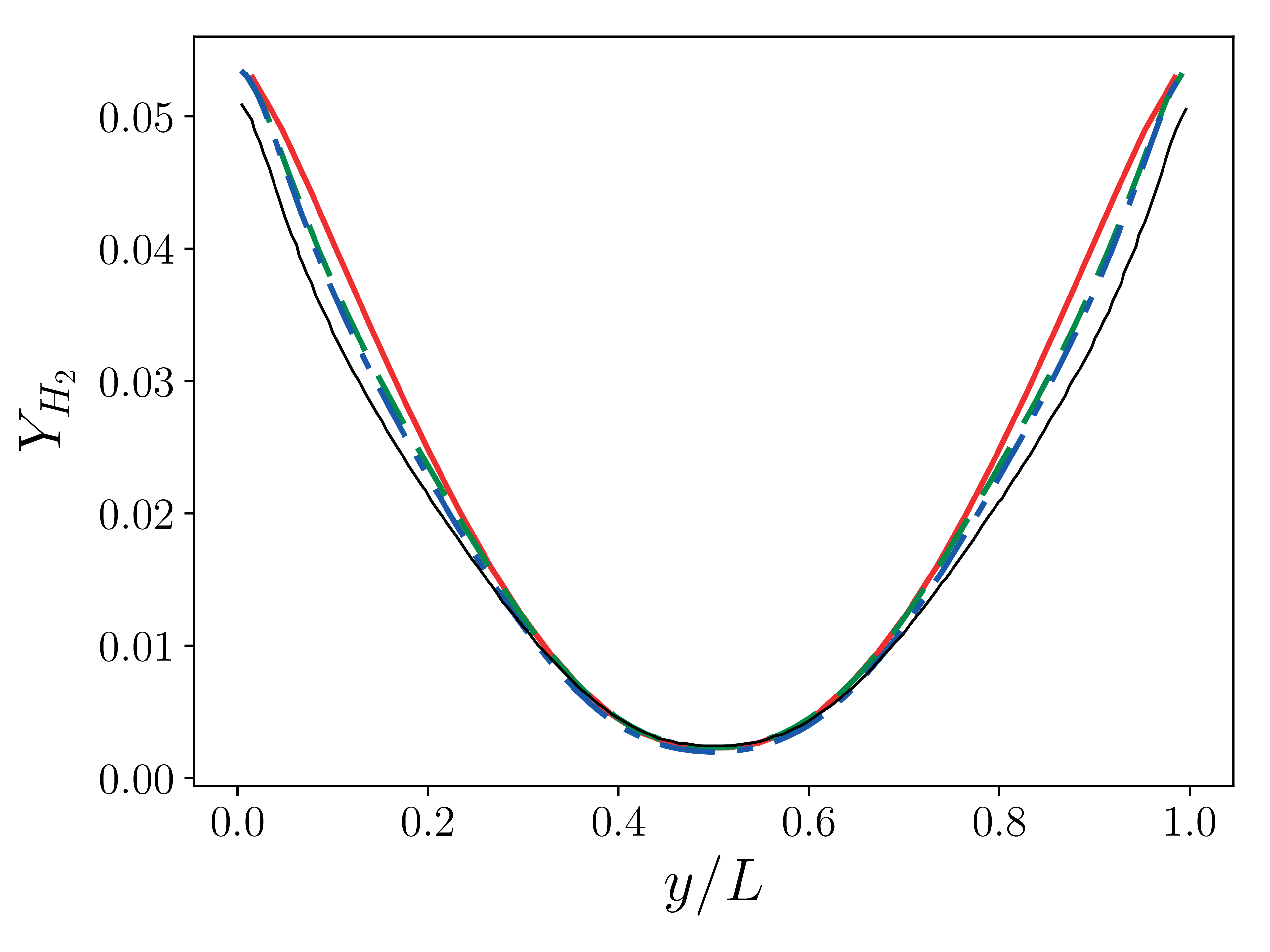
20 \(Y_{H_2}\) at \(t=5e-4 \tau\). Solid red: \(32^3\), dashed green \(64^3\), dash-dotted blue: \(128^3\), black: reference solution (DINO).
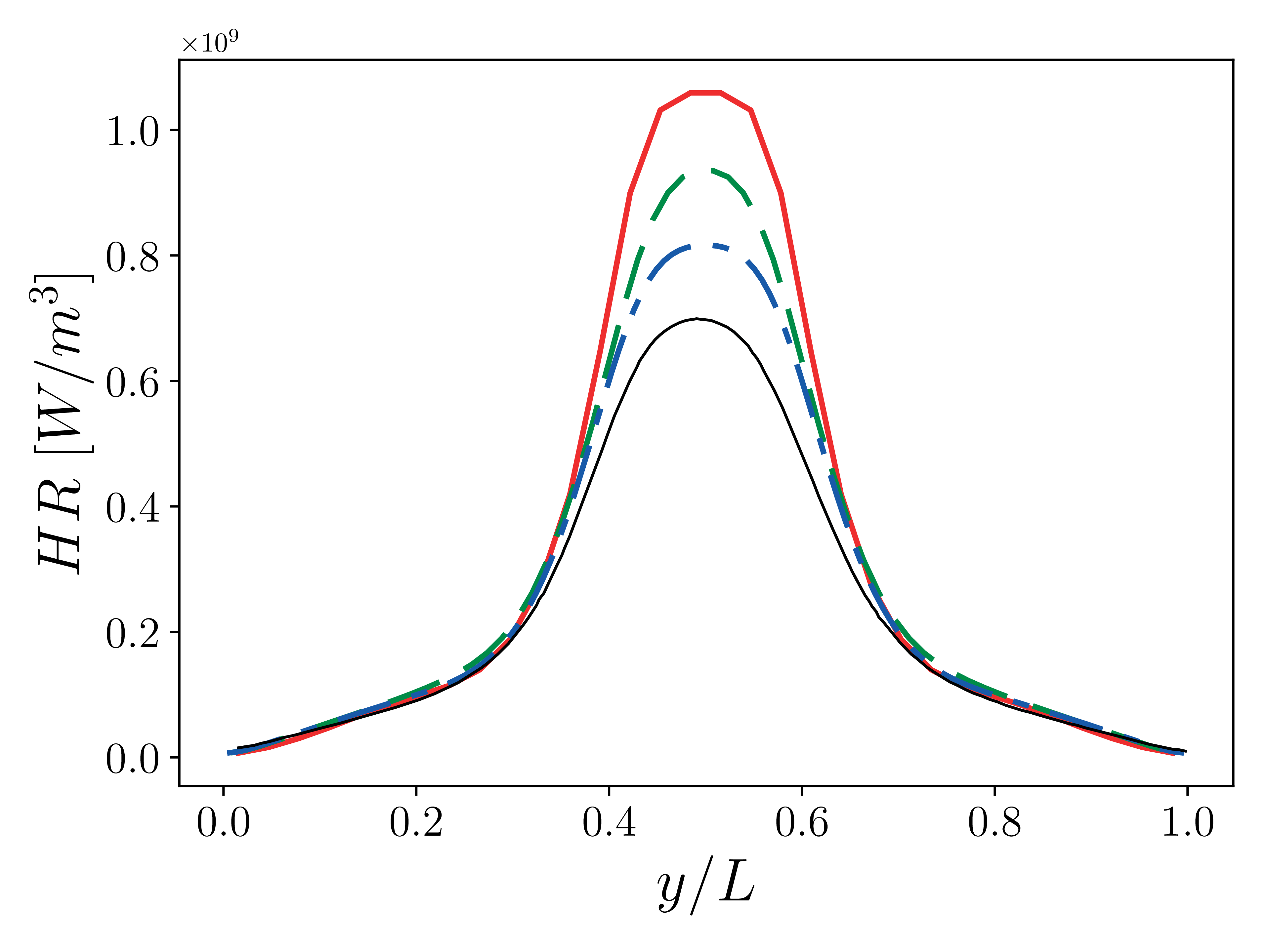
21 Heat release at \(t=5e-4 \tau\). Solid red: \(32^3\), dashed green \(64^3\), dash-dotted blue: \(128^3\), black: reference solution (DINO).
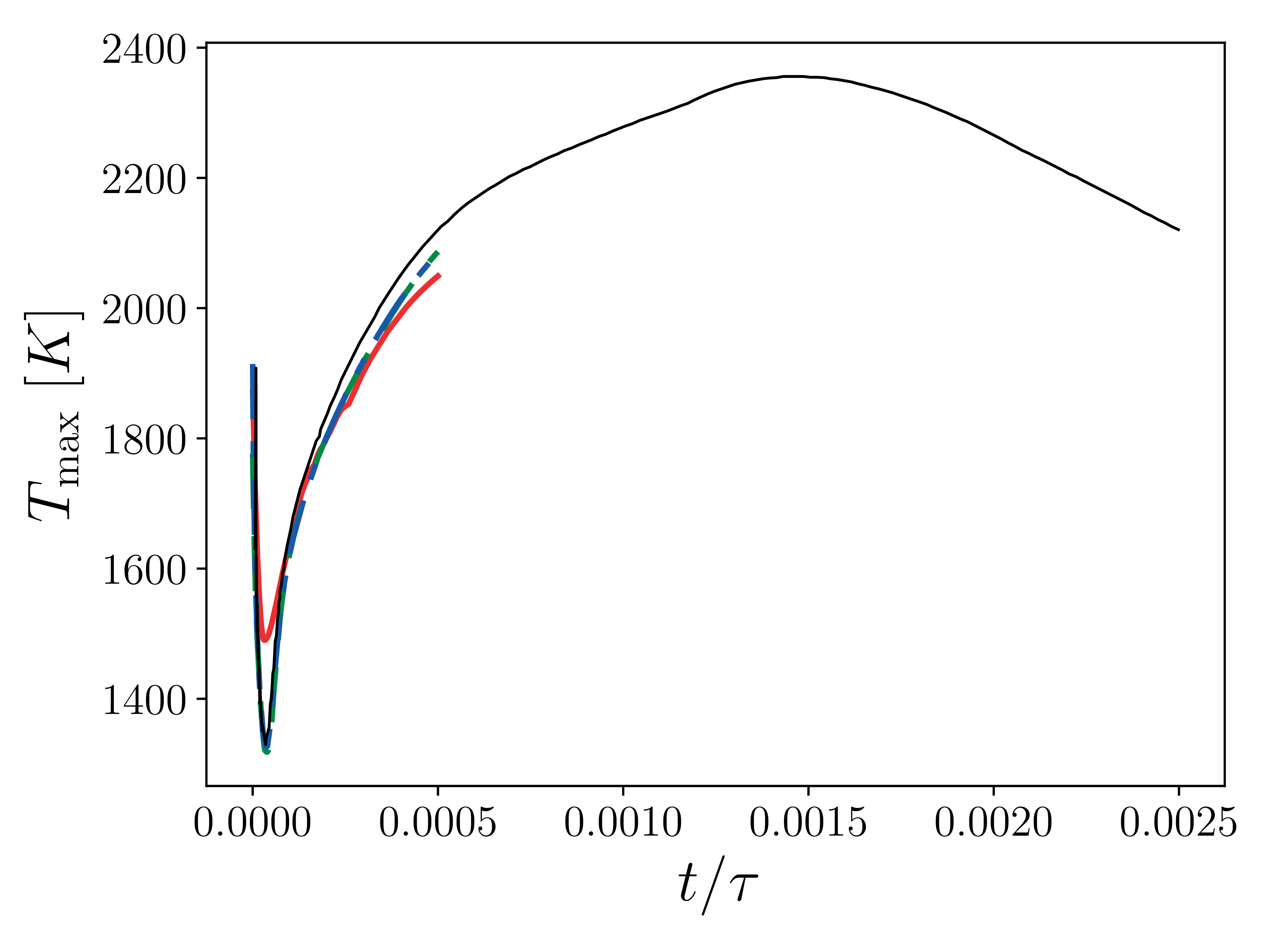
22 Maximum temperature in the domain as a function of time. Solid red: \(32^3\), dashed green \(64^3\), dash-dotted blue: \(128^3\), black: reference solution (DINO).
Note
We are not using the constant Lewis approximation that is prescribed in the workshop documentation. Instead we rely on transport coefficients resulting from PelePhysics. This may lead to discrepancies with the reference results.
Note
Because of computational constraints, we have not been able to perform higher resolution simulations that may show better convergence.
Counter flow diffusion flame
This test case simulated the well-known counter flow diffusion flame where fuel and oxidizer are injected head-on from opposite sides forming a stagnation region. The fuel-oxidizer diffusion in the stagnation region determines the flame location. The results from a PeleC simulation are shown in the figure below. The fuel (CH4) is injected from the left and air from the right. The temperature distribution indicates the flame location towards the oxidizer side. In a counter flow diffusion flame the key quantity to vary is the strain rate which is a function of mass flow rate of oxidizer and fuel streams. In this validation exercise, a series of strain rates will be simulated. Species and temperature profiles will be compared against the benchmark experimental data and well-established chemical kinetics solvers such as Cantera. The main motivation behind simulating a number of strain rates is to check the capability of PeleC to accurately reproduce the critical strain rate, known as the extinction limit.
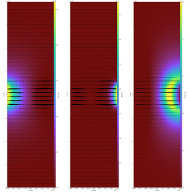
23 Fuel mass density is shown in left figure in g/cm3 (0(red)-1e-4(yellow)), oxygen mass density is shown in the middle figure (0 (red)-1e-5 (yellow)) and temperature is shown in right figure (1800K (red) - 2300 (yellow)) along with velocity vectors.
Note
A quantitative comparison with Cantera for varying strain-rates is work in progress
Counter flow premixed flame
Similar to the counter-flow diffusion flame, a common test case typically used to validate combustion codes is the opposed flow premixed flame. In contrast to the diffusion flame, in this case the opposing streams are composed of the same premixed fuel-air mixture. This case is typically referred to as the twin opposed flame because two flames are typically observed on the either side of the stagnation point. This case is particularly attractive since it allows for extinction at higher strain rates and simplified boundary conditions, unburnt mixture and temperature. The metric of comparison for the sake of validation would be species and temperature profiles. Well known solution profiles from experiments and highly resolved mesh converged 1-D Cantera simulations will be used to establish the accuracy of PeleC. In addition to profiles, a comparison of extinction strain rate will be also be made against the values obtained from 1-D Cantera simulation. Finally, we will also validate that PeleC simulations predict the correct premixed flame speed in the low strain rate limit.
Note
Not yet done.
Flame-Vortex interaction
The flame-vortex interaction test case provides a fundamental benchmark simulation to study interactions between the fluid flow and a flame in a controlled environment. In this simulation setup, a 2D flame front is initialized using profiles (velocity, species and temperature) from a 1-D premixed flame. Additionally, velocity field corresponding to a vortex field is superimposed using the Oseen vortex expression. This simulation is performed in an unsteady fashion with time evolution of flame area and stretch for varying ratios of vortex strength and laminar flame speed as the key metric for validation. Experimental data (Thiesset et. al, Proc. Combust. Inst. Volume 36, Issue 2, 2017, Pages 1843-1851) and data from a number of previously established simulation data will be used to validate PeleC.
Note
Not yet done.
Sandia Flame D
Flame D from the Sandia series of piloted methane/air turbulent jet flames (R. S. Barlow and J. H. Frank, Proc. Combust. Inst. Volume 27, 1998, Pages 1087-1095) is a canonical case for assessment of nonpremixed combustion models for LES in the literature and at the International Workshop on Measurement and Computation of Turbulent Flames (TNF). Extensive measurements of product species and temperature were taken at several locations in the flame, providing a wealth of data against which simulations can be validated. For validation of LES models for nonpremixed combustion in PeleC, conditional means and variances of temperature and species at several axial locations will be compared.
Note
Not yet done.
Premixed ignition kernel in isotropic turbulence
This test case is based on a set of DNS of spherical premixed Jet-A fuel/air kernels in decaying isotropic turbulence performed at Sandia National Laboratories (A. Krisman, T. Lu, and J. H. Chen, National Combustion Meeting, 2017, Paper #2E04). This test case will be used for validation of LES premixed combustion models in PeleC. This case allows for a priori model evaluation of local predictions of filtered reaction rates as well as a posteriori comparisons of global quantities of interest (kernel radius over time, successful or failed ignition).
Note
Not yet done.