Backward facing step anchored premixed flame

Introduction

The primary objective of PeleLMeX is to enable simulations of reactive flows on platforms ranging from small personal computers to Exascale supercomputers. This EB_BackwardStepFlame tutorial describes the case of a 2D laminar premixed methane/air flame anchored behind a backward facing step.

The goal of this tutorial is to introduce PeleLMeX users to more advanced reactive simulation setup as well as embedded boundaries.

Setting-up your environment

Getting a functioning environment in which to compile and run PeleLMeX is the first step of this tutorial. Follow the steps listed below to get to this point:

1. The first step is to get PeleLMeX and its dependencies. To do so, use a recursive git clone:

   git clone --recursive --shallow-submodules --single-branch https://github.com/AMReX-Combustion/PeleLMeX.git
   

   The --shallow-submodules and --single-branch flags are recommended for most users as they substantially reduce the size of the download by skipping extraneous parts of the git history. Developers may wish to omit these flags in order download the complete git history of PeleLMeX and its submodules, though standard git commands may also be used after a shallow clone to obtain the skipped portions if needed.

2. Move into the Exec folder containing your tutorial. To do so:

   cd PeleLMeX/Exec/RegTests/<CaseName>
   

   where <CaseName> is the name of your tutorial, e.g. HotBubble, FlameSheet, EB_BackwardStepFlame, EB_FlowPastCylinder, or TripleFlame.

You’re good to go!

Note

The makefile system is set up such that default paths are automatically set to the submodules obtained with the recursive git clone, however advanced users can set their own dependencies in the GNUmakefile for each case by updating the top-most lines as follows:

PELE_HOME     = <path_to_PeleLMeX>
AMREX_HOME        = <path_to_MyAMReX>
AMREX_HYDRO_HOME  = <path_to_MyAMReXHydro>
PELE_PHYSICS_HOME = <path_to_MyPelePhysics>
SUNDIALS_HOME     = <path_to_MySUNDIALS>

or directly through shell environment variables (using bash for instance):

export PELE_HOME=<path_to_PeleLMeX>
export AMREX_HOME=<path_to_MyAMReX>
export AMREX_HYDRO_HOME=<path_to_MyAMReXHydro>
export PELE_PHYSICS_HOME=<path_to_MyPelePhysics>
export SUNDIALS_HOME=<path_to_MySUNDIALS>

Note that using the first option will overwrite any environment variables you might have previously defined when using this GNUmakefile.

Case setup

A PeleLMeX case folder generally contains a minimal set of files to enable compilation, and the reader is referred to the FlameSheet tutorial Premixed flame sheet with harmonic perturbations for a more detailed description of PeleLMeX case setup. The case of interest for this tutorial can be found in PeleLMeX Exec folder:

Exec/RegTests/EB_BackwardStepFlame

Geometry, grid and boundary conditions

This simulation is performed on a 0.08x0.02 \(m^2\) 2D computational domain, with the bottom left corner located at (-0.01:-0.01) and the top right corner at (0.07:0.01). The flow is primarily aligned with the \(x\) direction with an Inflow (dirichlet) boundary on the \(x\)-low and Outflow (0-neumann) boundary on \(x\)-high. No-slip wall conditions are imposed the transverse direction. Finally a Cartesian coordinate system is used here. An overview of the computational domain is provided in Fig. 15.

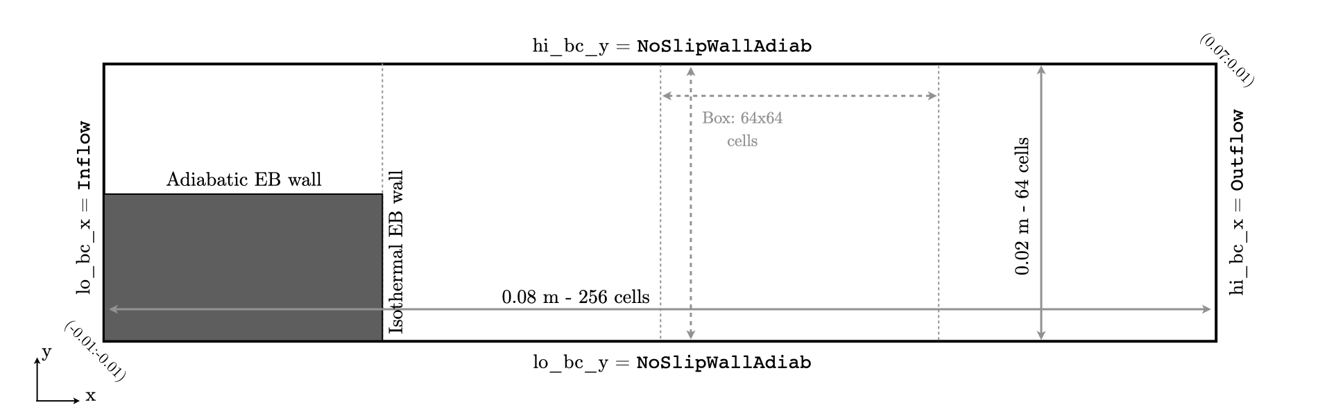
Fig. 15 : Setup of the computational domain for the backward facing step flame case.

All of the geometrical information can be specified the first two blocks of the input file (input.2d):

#---------------------- DOMAIN DEFINITION ------------------------
geometry.is_periodic = 0 0                  # For each dir, 0: non-perio, 1: periodic
geometry.coord_sys   = 0                    # 0 => cart, 1 => RZ
geometry.prob_lo     = -0.01   -0.01        # x_lo y_lo (z_lo)
geometry.prob_hi     =  0.07    0.01        # x_hi y_hi (z_hi)

#---------------------- BC FLAGS ---------------------------------
# Interior, Inflow, Outflow, Symmetry,
# SlipWallAdiab, NoSlipWallAdiab, SlipWallIsotherm, NoSlipWallIsotherm
peleLM.lo_bc = Inflow  NoSlipWallAdiab      # bc in x_lo y_lo (z_lo)
peleLM.hi_bc = Outflow NoSlipWallAdiab      # bc in x_hi y_hi (z_hi)

Note

Note that when running 2D simulations, it is not necessary to specify entries for the third dimension.

The base grid is decomposed into a 256x64 cell array with AMR initially not activated.

The refinement ratio between each level is set to 2 and PeleLMeX currently does not support refinement ratio of 4. Regrid operation will be performed every 5 steps. amr.n_error_buf specifies, for each level, the number of buffer cells used around the cell tagged for refinement, while amr.grid_eff describes the grid efficiency, i.e. how much of the new grid contains tagged cells. Higher values lead to tighter grids around the tagged cells. For more information on how these parameters affect grid generation, see the AMReX documentation.

All of those parameters are specified in the AMR CONTROL block:

#------------------------- AMR CONTROL ----------------------------
amr.n_cell          = 256 64           # Level 0 number of cells in each direction
amr.max_level       = 0                # maximum level number allowed
amr.ref_ratio       = 2 2 2 2          # refinement ratio
amr.regrid_int      = 5                # how often to regrid
amr.n_error_buf     = 2 2 2 2          # number of buffer cells in error est
amr.grid_eff        = 0.7              # what constitutes an efficient grid
amr.blocking_factor = 16               # block factor in grid generation
amr.max_grid_size   = 64               # maximum box size

Finally, this case uses Embedded Boundaries to represent the backward facing step. The EB is defined as a box on the lower-left corner of the domain. For such an easy geometry, a single AMReX native constructive solid geometry (CSG) object is sufficient. The box will extend from a point beyond the computational domain bottom left corner to (0.01:0.0). Because the intersection of the EB with the computational grid can lead to arbitrarily small cells, AMReX provides eb2.small_volfrac to set a cell volume fraction limit below which a cell is considered fully covered. In the present simulation, we will treat the EB as an isothermal boundary, with control over the wall temperature described in the next section.

#---------------------- EB SETUP ---------------------------------
eb2.geom_type = box
eb2.box_lo =    -0.02   -0.02
eb2.box_hi =     0.01     0.0
eb2.box_has_fluid_inside = 0
eb2.small_volfrac   = 1.0e-4
peleLM.isothermal_EB = 1

Note

When EBs intersect with the domain boundary, it is important to ensure that the EB definition extends slightly beyond the domain boundaries to provide EB structure data in the domain ghost cells.

Problem specifications

The problem setup is mostly contained in the three C++ source/header files described in Premixed flame sheet with harmonic perturbations. The user parameters are gathered in the struct defined in pelelmex_prob_parm.H:

struct ProbParm
{
    amrex::Real T_mean = 298.0_rt;
    amrex::Real P_mean = 101325.0_rt;
    amrex::Real Y_fuel = 0.0445_rt;
    amrex::Real Y_o2   = 0.223_rt;
    amrex::Real T_hot  = 1800.0_rt;
    amrex::Real Twall  = 300.0_rt;
    amrex::Real meanFlowMag = 0.0;
};

• T_mean : inlet and initial gas temperature

• P_mean : initial thermodynamic pressure

• Y_fuel : inlet and initial fuel (CH4) mass fraction

• Y_oxid : inlet and initial oxidizer (O2) mass fraction

• T_hot : initial temperature in the step wake

• T_wall : EB-wall temperature

• meanFlowMag : inlet \(x\) velocity

The initial solution consists of a premixed methane/air mixture in the upper part of the domain and pure hot air in the wake of the step. The default parameters provided above are overwritten using AMReX ParmParse in pelelmex_prob.cpp and the initial/boundary conditions implemented in pelelmex_prob.H.

In addition to these three C++ files, an extra header is needed in the present case compared to Premixed flame sheet with harmonic perturbations : EBUserDefined.H. This file is necessary to specify more complex EB geometries (not the case here) and to prescribe EB isothermal wall condition. It contains three functions:

• EBUserDefined() : can be used to provide a user-defined geometry. It is left empty in the present case.

• setEBState() : takes in the EB face center coordinates and return a vector for the entire state vector. For isothermal walls, only the TEMP component is required.

• setEBType() : even though peleLM.isothermal_EB=1 is activated, the user can locally decide to use an adiabatic wall on part of the EB. To do so, this function takes in the EB face center coordinates and return a Real flag that should be set to 1.0 on isothermal areas and 0.0 on adiabatic areas. The flag is later used to pre-multiply the thermal diffusivity effectively zeroing the thermal flux where the flag is 0.0.

In the present case, we set the EB temperature to T_wall everywhere on the EB in setEBState() but the EB flag is only set to 1.0 on the vertical EB faces (\(x\) normal) such that the top of the EB box is adiabatic.

Numerical parameters

The PeleLM CONTROL block contains a few of the PeleLMeX algorithmic parameters. Many more unspecified parameters are relying on their default values which can be found in PeleLMeX controls. Of particular interest are the peleLM.sdc_iterMax parameter controlling the number of SDC iterations (see The PeleLMeX Model for more details on SDC in PeleLMeX) and the peleLM.num_init_iter one controlling the number of initial iteration the solver will do after initialization to obtain a consistent pressure and velocity field.

Building the executable

Now that we have reviewed the basic ingredients required to setup the case, it is time to build the PeleLMeX executable. Although both GNUmake and CMake are available, it is advised to use GNUmake. The GNUmakefile file provides some compile-time options regarding the simulation we want to perform. The first few lines specify the paths towards the source codes of PeleLMeX, AMReX, AMReX-Hydro and PelePhysics, overwriting any environment variable if necessary, and might have been already updated in Setting-up your environment earlier.

The next few lines specify AMReX compilation options and compiler selection:

# AMREX
DIM             = 2
DEBUG           = FALSE
PRECISION       = DOUBLE
VERBOSE         = FALSE
TINY_PROFILE    = FALSE
USE_EB          = TRUE
USE_HYPRE       = FALSE

# Compilation
COMP            = gnu
USE_MPI         = TRUE
USE_OMP         = FALSE
USE_CUDA        = FALSE
USE_HIP         = FALSE
USE_SYCL        = FALSE

It allows users to specify the number of spatial dimensions (2D), activate the compilation of the EB aware AMReX source code, trigger debug compilation and other AMReX options. The compiler (gnu) and the parallelism paradigm (in the present case only MPI is used) are then selected. Note that on OSX platform, one should update the compiler to llvm.

The user also needs to make sure the additional C++ header employed to define the EB state is included in the build:

# PeleLMeX
CEXE_headers    += EBUserDefined.H

In PeleLMeX, the chemistry model (set of species, their thermodynamic and transport properties as well as the description of their of chemical interactions) is specified at compile time. Chemistry models available in PelePhysics can used in PeleLMeX by specifying the name of the folder in PelePhysics/Mechanisms containing the relevant files, for example:

Chemistry_Model = drm19

Here, the model drm19 contains 21 species and describe the chemical decomposition of methane. The user is referred to the PelePhysics documentation for a list of available mechanisms and more information regarding the EOS, chemistry and transport models specified:

Eos_Model       := Fuego
Transport_Model := Simple

Finally, PeleLMeX utilizes the chemical kinetic ODE integrator CVODE. This Third Party Library (TPL) is shipped as a submodule of the PeleLMeX distribution and can be readily installed through the makefile system of PeleLMeX. To do so, type in the following command:

make -j4 TPL

Note that the installation of CVODE requires CMake 3.23.1 or higher.

You are now ready to build your first PeleLMeX executable!! Type in:

make -j4

The option here tells make to use up to 4 processors to create the executable (internally, make follows a dependency graph to ensure any required ordering in the build is satisfied). This step should generate the following file (providing that the build configuration you used matches the one above):

PeleLMeX2d.gnu.MPI.ex

You’re good to go!

Checking the initial conditions

It is always a good practice to check the initial conditions. To do so, run the simulation specifying an amr.max_step of 0. Open the input.2d with your favorite editor and update the following parameters

#---------------------- Time Stepping CONTROL --------------------
amr.max_step      = 0             # Maximum number of time steps

Since we’ve set the maximum number of steps to 0, the solver will exit after the initial solution is obtained. Let’s run the simulation with the default problem parameter listed in the input file. To do so, use:

./PeleLMeX2d.gnu.MPI.ex input.2d-regt

A variety of information is printed to the screen:

1. AMReX/SUNDIALs initialization along with the git hashes of the various subrepositories

2. A summary of the PeleLMeX state components

3. Initial projection and initial iterations.

4. Saving the initial solution to plt00000 file.

Use Amrvis, Paraview or yt to visualize the plot file. Using Amrvis, the solution should look similar to Fig. 16.

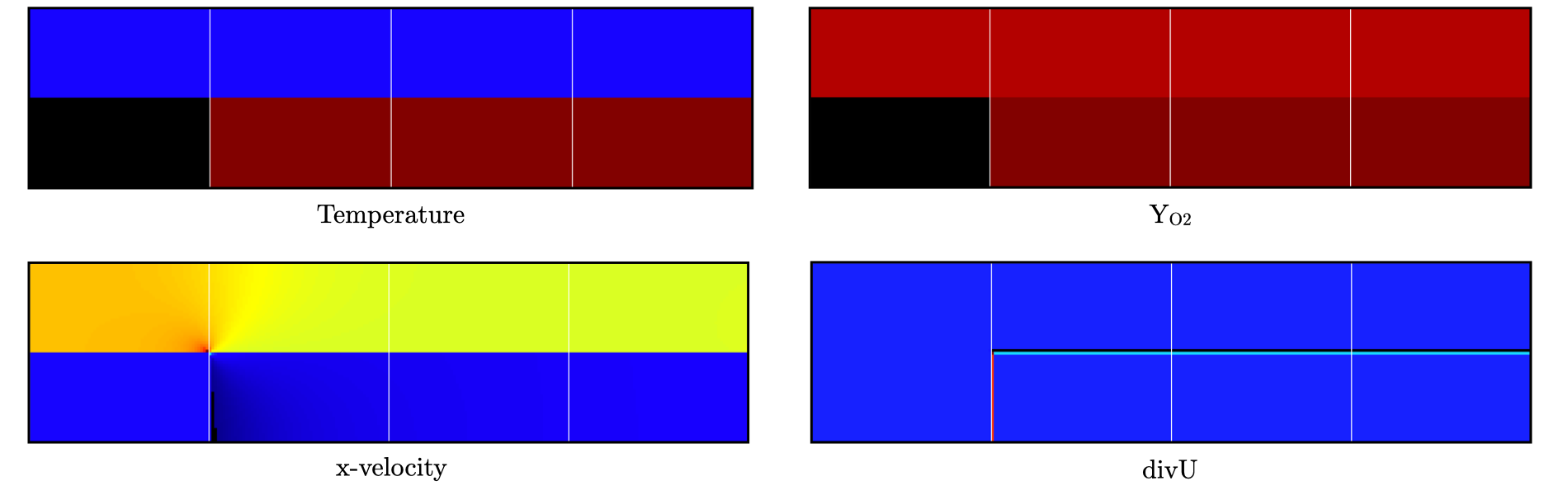
Fig. 16 : Contour plots of temperature, O2 mass fraction, \(x\)-velocity component and divergence constraint after initialization.

Note that in PeleLMeX, EB-covered regions are set to zero in plotfiles. Hot gases are found in the wake of the EB as expected, with a slightly higher O2 mass fraction compared to the upper part of the domain where CH4 is present in the mixture. The velocity field results from the initial projection, which uses the divergence constraint. The later is negative close to the isothermal EB because the cold EB leads to an increase of density. divU is also non zero at the interface between the incoming fresh gases and the hot air due to heat diffusion.

Advance the solution on coarse grid

Let’s now advance the solution for 250 steps, using only the base grid and the default time stepping parameters. To do so, ensure that:

amr.max_step = 250

Additionally, make sure that amr.check_int is set to a positive value to trigger writing a checkpoint file from which to later restart the simulation. If available, use more than one MPI rank to run the simulation and redirect the standard output to a log file using:

mpirun -n 4 ./PeleLMeX2d.gnu.MPI.ex input.2d > logInitCoarse.dat &

Using 4 MPI ranks, it takes about 200 seconds to complete. A typical PeleLMeX stdout for a time step now looks like:

====================   NEW TIME STEP   ====================
Est. time step - Conv: 9.42747435e-06, divu: 0.0002752479251
STEP [125] - Time: 5.072407773e-05, dt 5.072441746e-06
  SDC iter [1]
  SDC iter [2]
>> PeleLM::Advance() --> Time: 0.877052

clearly showing the use of 2 SDC iterations. The first line at each step provides the time step constraint from the CFL condition (Conv:) and from the density change condition (divu:). Since an initial dt_shrink was applied upon initialization, the current step is smaller than the CFL but progressively increases over the course of the simulation, eventually reaching the CFL constrained step size after 133 steps. After 250 steps, the simulation time is around 1.25 ms and the step size is of the order of 10 \(\mu s\).

Visualizing the plt00250 file, we can see that the solution has evolved, with a vortex propagating downstream along the flame surface, while intermediate species can be found. Looking at the heat release rate and the H2 mass fraction, we can see that the flame front is very poorly resolved. The density along the isothermal EB also increased under the effect of the cold wall.

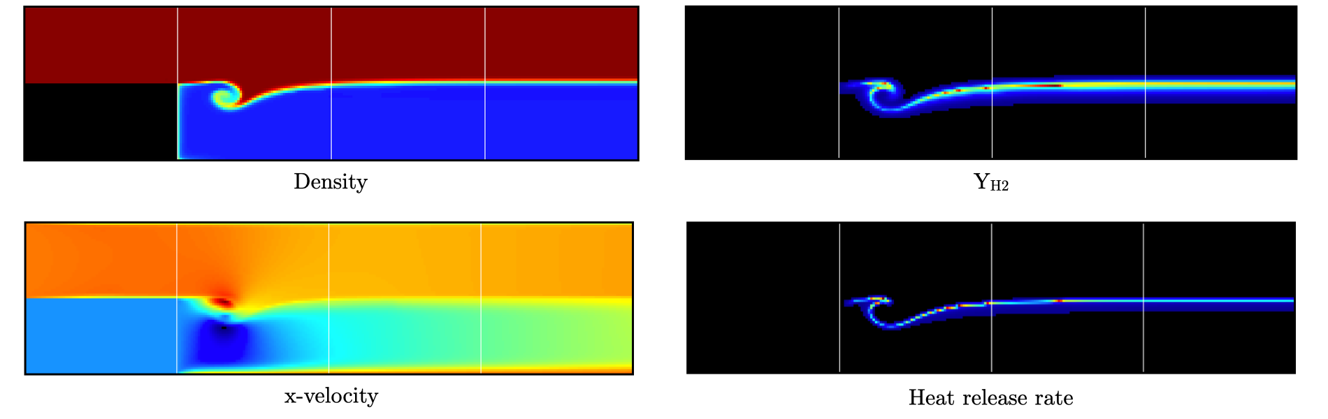
Fig. 17 : Contour plots of density, H2 mass fraction, \(x\)-velocity component and heat release rate after 250 steps.

In order to illustrate one of PeleLMeX failure modes, we will now continue the simulation for another 50 steps, starting from chk00250, while increasing the CFL number to 0.6. Update the following keys in the input file:

#---------------------- Time Stepping CONTROL --------------------
amr.max_step = 300                          # Maximum number of time steps
...
amr.cfl = 0.6                               # CFL number for hyperbolic system

...
#---------------------- IO CONTROL -------------------------------
amr.restart = chk00250                      # Restart checkpoint file

and restart the simulation:

mpirun -n 4 ./PeleLMeX2d.gnu.MPI.ex input.2d > logFail.dat &

The simulation will proceed, with the step size progressively increasing due to the higher CFL and changes to the velocity field, but after ~30 steps PeleLMeX will fail with the following error:

====================   NEW TIME STEP   ====================
Est. time step - Conv: 1.550410967e-05, divu: 5.712875519e-05
STEP [282] - Time: 0.001701680124, dt 1.550410967e-05
  SDC iter [1]
  SDC iter [2]
amrex::Abort::3::Aborting from CVODE !!!
SIGABRT
From CVODE: At t = 1.43329e-05, mxstep steps taken before reaching tout.

The combination of large time step size and poor flame resolution leads to a very stiff chemical system, where fuel, oxidizer, intermediate species and heat are mixed within the cell averaged state representation associated with finite volume. The CVODE error clearly states that the internal sub-stepping of the ODE integrator was not able to integrate past 1.43329e-05. This is an indication that the CFL constraint is too loose compared to chemical stiffness, even though a implicit solve is performed. This generally occurs in laminar flows with coarse resolution, but could also occurs in midly turbulent flames with stiff chemical mechanisms. If you plan on pushing the simulation forward without adding refinement, it is advised to reduce CFL to smaller value.

Refine the simulation

Instead, let’s add a first level of refinement and keep the CFL at a value of 0.6, while restarting again from chk00250. Enable AMR refinement by increasing the amr.max_level:

#---------------------- AMR CONTROL ------------------------------
...
amr.max_level       = 1                     # maximum level number allowed
...

And increase the maximum number of steps to 500:

#---------------------- Time Stepping CONTROL --------------------
amr.max_step = 500                          # Maximum number of time steps
...

Restart the simulation:

mpirun -n 4 ./PeleLMeX2d.gnu.MPI.ex input.2d > log1AMR.dat &

Using 4 MPI ranks, the simulation takes approximately 13 mn, so plenty of time to get a warm beverage. Looking at the solution after 500 steps (~3.2 ms), fine boxes can be found around the EB and along the flame. This is consistent with PeleLMeX default behavior which consists of refining the EB up to the finest level, and the refinement criterion specified in the Refinement CONTROL block near the end of the input file:

#---------------------- Refinement CONTROL------------------------
amr.refinement_indicators = gradT
amr.gradT.max_level     = 3
amr.gradT.adjacent_difference_greater = 100
amr.gradT.field_name    = temp

This input block triggers cell tagging for refinement if the adjacent cell in any directions has a temperature difference larger than 100 K. Because the of the blocking factor and the grid efficiency value, most of the lower part of the computational domain is actually refined to Level 1.

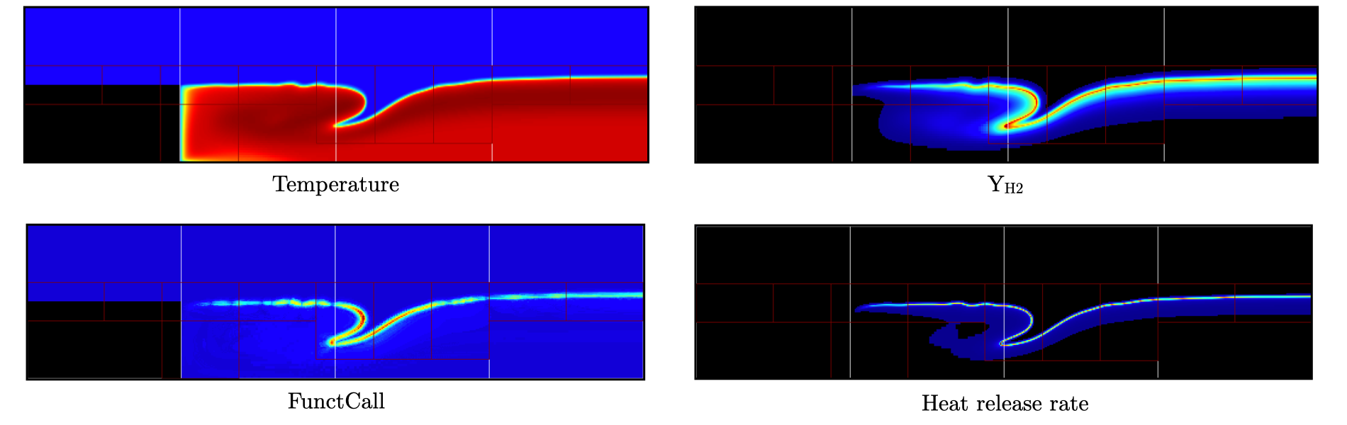
Fig. 18 : Contour plots of temperature, H2 mass fraction, chemistry functCall and heat release rate after 500 steps, using 1 level of AMR.

The functCall variable corresponds to the number of time CVODE called the chemical right-hand-side function and is a good indicator of the computational cost of the integration of the implicit chemical system. Values up to ~70 can be found in the vicinity of the flame front while values < 10 are found outside of the flame, highligthind the high spatial heterogeneity of combustion simulations. Even though a flame has established, the recirculation zone in the wake of the backward facing step is still mostly filled with the initial hot air mixture. Let’s restart the simulation again for another 500 steps using the same setup, only adding a few extra parameters:

• increase PeleLMeX verbose peleLM.v = 2 is order to get more information about the advance function.

• add following to the list of derived variables stored in plotfile (amr.derive_plot_vars): mixture_fraction, progress_variable.

In order for the mixture fraction and progress variable to be properly define, users must provide the composition of the fuel and oxidizer streams, and the cold and hot mixture states, respectively. To do so, update the following block:

#---------------------- Derived CONTROLS -------------------------
peleLM.fuel_name = CH4
peleLM.mixtureFraction.format = Cantera
peleLM.mixtureFraction.type   = mass
peleLM.mixtureFraction.oxidTank = O2:0.233 N2:0.767
peleLM.mixtureFraction.fuelTank = CH4:1.0
peleLM.progressVariable.format = Cantera
peleLM.progressVariable.weights = CO:1.0 CO2:1.0
peleLM.progressVariable.coldState = CO:0.0 CO2:0.0
peleLM.progressVariable.hotState = CO:0.003 CO2:0.122

Update the amr.restart and amr.max_step to chk00500 and 1000, respectively and restart the simulation:

mpirun -n 4 ./PeleLMeX2d.gnu.MPI.ex input.2d > log1AMRcnt.dat &

Once again, the simulation takes approximately 30 mn to complete. At this point, the flame is fairly well established in the downstream part of the domain, but the mixture_fraction field can clearly show that hot air is still trapped in the recirculation. Because of the cold EB wall, the flame is detached from the EB wall and stabilized by an ignition mechanism in the shear layer between the incoming fressh, flammable mixture and the recirculated hot gases. A look at the heat release rate field will show that the flame is still highly under-resolved. Let’s continue the simulation with an additional level of refinement. However, we could now want to keep the next level on the flame only. However, AMReX (and thus PeleLMeX) does not enable coarse-fine boundaries to intersect the EB. In other words, a continuous EB surface must be at the same level. But this level doesn’t have to be the finest level used in the simulation. In order to control the EB refinement level, let’s add the following lines to the Refinement CONTROL block:

peleLM.refine_EB_type = Static
peleLM.refine_EB_max_level = 1
peleLM.refine_EB_buffer = 2.0

These input keys will initiate a de-refining mechanism where local refinement triggered by other tagging criterions will be removed above the level specified (1 in the present case), preventing coarse-fine boundary from intersecting the EB. The last keyword is a factor controlling how far from the EB the de-refining is applied is is useful for deep AMR hierarchy with complex geometries where proper nesting of finer levels might extend the reach of an AMR level far beyond the region where tagging for that level is triggered. Because PeleLMeX operates without subcycling, the step size decreases as we add refinement levels. As such, we can increase slightly the CFL number (but no higher than 0.9) because we will now advance at a step size much small than the ones where we experienced CVODE integration issues earlier in this tutorial. Let’s set amr.cfl=0.7, increase the amr.max_level=2 and restart the simulation for another 200 steps (updating again the restart file and max step).

The simulation with take about 22 mn on 4 MPI ranks. A typical log file step with regridding will look like:

====================   NEW TIME STEP   ====================
Regridding...
Remaking level 1
Remaking level 2
Resetting fine-covered cells mask
Est. time step - Conv: 4.947086647e-06, divu: 3.473512656e-05
STEP [1195] - Time: 0.008834263469, dt 4.947086647e-06
  SDC iter [1]
  - oneSDC()::MACProjection()   --> Time: 0.241061
  - oneSDC()::ScalarAdvection() --> Time: 0.141316
  - oneSDC()::ScalarDiffusion() --> Time: 1.351
  - oneSDC()::ScalarReaction()  --> Time: 1.368832
  SDC iter [2]
  - oneSDC()::Update t^{n+1,k}  --> Time: 0.53102
  - oneSDC()::MACProjection()   --> Time: 0.136435
  - oneSDC()::ScalarAdvection() --> Time: 0.1527
  - oneSDC()::ScalarDiffusion() --> Time: 1.07304
  - oneSDC()::ScalarReaction()  --> Time: 1.18373
  - Advance()::VelocityAdvance  --> Time: 0.325139
>> PeleLM::Advance() --> Time: 7.528655

The increased verbose explicitly shows the various pieces of PeleLMeX advance function and their computational cost. In the present case, diffusion and reaction are about the same computational cost, 5 to 10 times more expensive than the other parts of the algorithm. Both AMR levels where updated at the beginning of the time steps. With the additional refinement, the flame front is now resolved with a few grid cells (but still below DNS requirements).

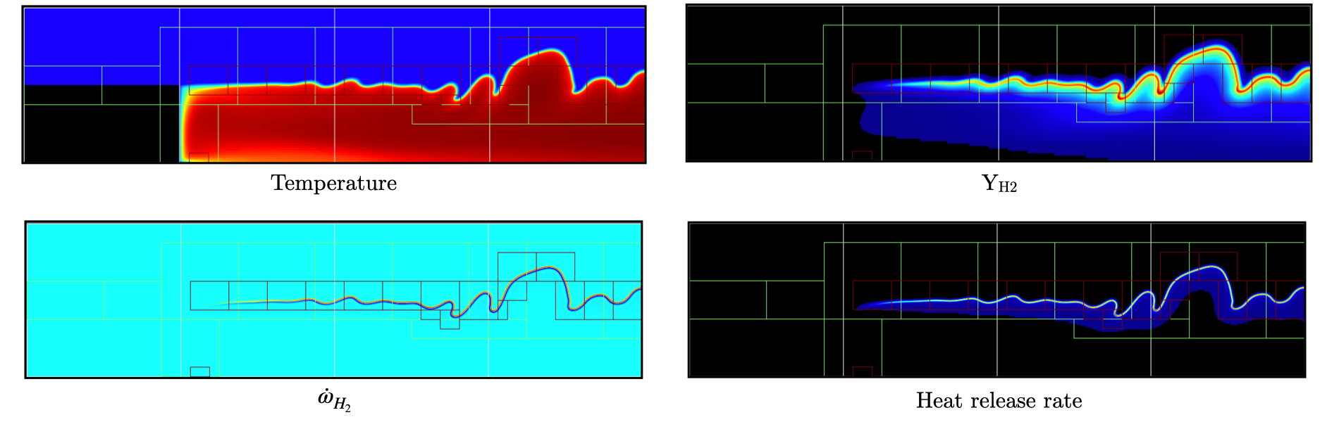
Fig. 19 : Contour plots of temperature, H2 mass fraction, H2 production rate and heat release rate after 1200 steps, using 2 levels of AMR.

The AMR level 2 is clearly distant from the EB and concentrated mostly on the flame surface (except a small box at the bottom of the recirculation zone which could be alleviated by using a refinement criterion based a flame intermediate species rather than temperature difference). Let’s conclude this tutorial by another two AMR levels and provide an example of PeleLMeX runtime diagnostics. We will restart the simulation for another 10 steps with a amr.max_level=3. increasing the verbose to peleLM.v = 3 and defining a couple of diagnostics.

We are interested in evaluating how much the premixed flame near the EB wall differs from the one further downstream. To provide quantitative data, we will compute conditional averaged value of reaction markers and intermediate species as function of the progress variable. We can do this by defining the same diagnostics but extracted on the upstream and downstream regions of the computational domain as follows:

peleLM.diagnostics = CondMeanUp CondMeanDown
peleLM.CondMeanUp.type = DiagConditional
peleLM.CondMeanUp.int  = 10
peleLM.CondMeanUp.filters = lowX middleY
peleLM.CondMeanUp.lowX.field_name = x
peleLM.CondMeanUp.lowX.value_inrange = 0.011 0.035
peleLM.CondMeanUp.middleY.field_name = y
peleLM.CondMeanUp.middleY.value_inrange = -0.005 0.005
peleLM.CondMeanUp.conditional_type = Average
peleLM.CondMeanUp.nBins = 40
peleLM.CondMeanUp.condition_field_name = progress_variable
peleLM.CondMeanUp.field_names = HeatRelease Y(H2) Y(CO) I_R(CH4) I_R(H2)

peleLM.CondMeanDown.type = DiagConditional
peleLM.CondMeanDown.int  = 10
peleLM.CondMeanDown.filters = highX middleY
peleLM.CondMeanDown.highX.field_name = x
peleLM.CondMeanDown.highX.value_inrange = 0.035 0.07
peleLM.CondMeanDown.middleY.field_name = y
peleLM.CondMeanDown.middleY.value_inrange = -0.005 0.005
peleLM.CondMeanDown.conditional_type = Average
peleLM.CondMeanDown.nBins = 40
peleLM.CondMeanDown.condition_field_name = progress_variable
peleLM.CondMeanDown.field_names = HeatRelease Y(H2) Y(CO) I_R(CH4) I_R(H2)

Using different filters option, the first diagnostic will extract data from the region comprised in the \(x\) [0.011:0.035] while the second one further downstream in \(x\) [0.035:0.07].

Let’s restart the simulation for another 10 steps (updating the restart file and max step). The additional verbose allows to get an idea of the number of cells in the simulation:

====================   NEW TIME STEP   ====================
Regridding...
Remaking level 1
with 37120 cells, over 56.640625% of the domain
Remaking level 2
with 67072 cells, over 25.5859375% of the domain
Remaking level 3
with 117760 cells, over 11.23046875% of the domain
Making new level 4 from coarse
with 189696 cells, over 4.522705078% of the domain
Resetting fine-covered cells mask
Est. time step - Conv: 1.221962099e-06, divu: 3.340072395e-05
STEP [1205] - Time: 0.008871299457, dt 1.221962099e-06
...

Showing that the finest level contains as many cells as the next two coarser levels on only a fraction of the space. Two additional ASCII files containing the conditional averaged data have been created and using for example gnuplot, the user can compare the conditional averaged heat release rate between the upstream and downstream region of the flame.

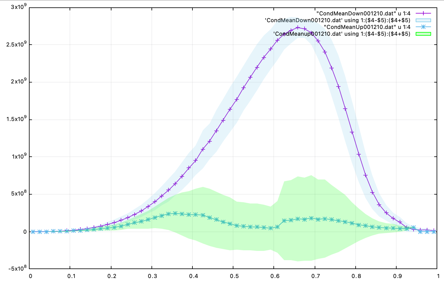
Fig. 20 : Conditional average and standard deviation of heat release rate after 1210 steps, using 4 levels of AMR.

Note that for this analysis to be relevant, we would need to run the simulation longer to completely remove the effect of the initial hot air still trapped in the recirculation zone at this point and largely affecting the upstream average data.