Rising light bubble
Introduction
At the core of PeleLMeX algorithm is a variable-density, low Mach number Navier-Stokes solver based
on a fractional step approach. This short HotBubble tutorial presents the case of a rising light bubble under
the influence of a gravity field, which exercise this algorithm without the added complexity
of chemical reactions or embedded boundaries.
Setting-up your environment
Getting a functioning environment in which to compile and run PeleLMeX is the first step of this tutorial. Follow the steps listed below to get to this point:
The first step is to get PeleLMeX and its dependencies. To do so, use a recursive git clone:
git clone --recursive --shallow-submodules --single-branch https://github.com/AMReX-Combustion/PeleLMeX.git
The
--shallow-submodulesand--single-branchflags are recommended for most users as they substantially reduce the size of the download by skipping extraneous parts of the git history. Developers may wish to omit these flags in order download the complete git history of PeleLMeX and its submodules, though standardgitcommands may also be used after a shallow clone to obtain the skipped portions if needed.Move into the Exec folder containing your tutorial. To do so:
cd PeleLMeX/Exec/RegTests/<CaseName>
where <CaseName> is the name of your tutorial, e.g.
HotBubble,FlameSheet,EB_BackwardStepFlame,EB_FlowPastCylinder, orTripleFlame.
You’re good to go!
Note
The makefile system is set up such that default paths are automatically set to the submodules obtained with the recursive git clone, however advanced users can set their own dependencies in the GNUmakefile for each case by updating the top-most lines as follows:
PELE_HOME     = <path_to_PeleLMeX>
AMREX_HOME        = <path_to_MyAMReX>
AMREX_HYDRO_HOME  = <path_to_MyAMReXHydro>
PELE_PHYSICS_HOME = <path_to_MyPelePhysics>
SUNDIALS_HOME     = <path_to_MySUNDIALS>
or directly through shell environment variables (using bash for instance):
export PELE_HOME=<path_to_PeleLMeX>
export AMREX_HOME=<path_to_MyAMReX>
export AMREX_HYDRO_HOME=<path_to_MyAMReXHydro>
export PELE_PHYSICS_HOME=<path_to_MyPelePhysics>
export SUNDIALS_HOME=<path_to_MySUNDIALS>
Note that using the first option will overwrite any environment variables you might have previously defined when using this GNUmakefile.
Case setup
A PeleLMeX case folder contains a minimal set of files to enable compilation, and the reader is referred to the FlameSheet tutorial Premixed flame sheet with harmonic perturbations for a more detailed description of PeleLMeX case setup. The case of interest for this tutorial can be found in PeleLMeX Exec folder:
Exec/RegTests/HotBubble
Geometry, grid and boundary conditions
This simulation is performed on a 0.016x0.032 \(m^2\) 2D computational domain,
with the bottom left corner located at (0.0:0.0) and the top right corner at (0.016:0.032).
Two versions of that domain will be considered: 1) a 2D-cartesian case, 2) a 2D-RZ
case where the \(x\)-low is the symmetry axis of the azimuthally homogeneous case. In both cases, the
\(x\)-low boundary is treated as symmetry BC while \(x\)-high is treated as an adiabatic slip wall,
the \(y\)-low boundary is treated as an adiabatic slip wall, while the \(y\)-high boundary is an Outflow.
All of the geometrical information can be specified the first two blocks of the input file (input.2d-regt_sym):
#----------------------DOMAIN DEFINITION------------------------
geometry.is_periodic = 0 0                  # For each dir, 0: non-perio, 1: periodic
geometry.coord_sys   = 0                    # 0 => cart, 1 => RZ
geometry.prob_lo     = 0.0 0.0              # x_lo y_lo (z_lo)
geometry.prob_hi     = 0.016 0.032          # x_hi y_hi (z_hi)

# >>>>>>>>>>>>>  BC FLAGS <<<<<<<<<<<<<<<<
# Interior, Inflow, Outflow, Symmetry,
# SlipWallAdiab, NoSlipWallAdiab, SlipWallIsotherm, NoSlipWallIsotherm
peleLM.lo_bc = Symmetry      SlipWallAdiab
peleLM.hi_bc = SlipWallAdiab Outflow
In the 2D-RZ case (input.2d-regt_symRZ), the geometry.coord_sys is updated to 1 to trigger the use of a polar
coordinates system.
Note
Note that when running 2D simulations, it is not necessary to specify entries for the third dimension.
The base grid is decomposed into a 64x128 cell array with AMR triggered up to level 2.
The refinement ratio between each level is set to 2 and PeleLMeX currently does not support
refinement ratio of 4. Regrid operation will be performed every 5 steps. amr.n_error_buf specifies,
for each level, the number of buffer cells used around the cell tagged for refinement, while amr.grid_eff
describes the grid efficiency, i.e. how much of the new grid contains tagged cells. Higher values lead
to tighter grids around the tagged cells. For more information on how these parameters affect grid generation,
see the AMReX documentation.
All of those parameters are specified in the AMR CONTROL block:
#------------------------- AMR CONTROL ----------------------------
amr.n_cell          = 64 128         # Level 0 number of cells in each direction
amr.v               = 1              # AMR verbose
amr.max_level       = 2              # maximum level number allowed
amr.ref_ratio       = 2 2 2 2        # refinement ratio
amr.regrid_int      = 5              # how often to regrid
amr.n_error_buf     = 1 1 2 2        # number of buffer cells in error est
amr.grid_eff        = 0.7            # what constitutes an efficient grid
amr.blocking_factor = 16             # block factor in grid generation (min box size)
amr.max_grid_size   = 128            # max box size
Problem specifications
The problem setup is mostly contained in the two C++ source/header files described in Premixed flame sheet with harmonic perturbations.
The user parameters are gathered in the struct defined in pelelmex_prob.H:
struct ProbParm : public ProbParmDefault
{
    amrex::Real P_mean        = 101325.0;
    amrex::Real T_mean        = 300.0;
    amrex::Real T_bubble      = 600.0;
    amrex::Real bubble_rad    = 0.005;
    amrex::Real bubble_y0     = 0.01;
    int         bubble_is_mix = 0;
    int           is_sym      = 0;
};
P_mean: initial thermodynamic pressureT_mean: the ambient gas temperatureT_bubble: the bubble gas temperaturebubble_rad: the radius of the light bubblebubble_y0: the initial position of the bubble in the \(y\) directionbubble_is_mix: a flag to switch to a mixture-based density change in the bubbleis_sym: a flag to indicate that the initial conditions are for a \(x\)-low symmetric case.
The initial solution consists of air at the pressure/temperature specified by the user, with a bubble
of a different temperature/mixture intended to be lighter such that the bubble will rise under the
influence of gravity. Note that the user can easily reverse the problem with a heavier bubble.
The default parameters provided above are overwritten using AMReX ParmParse in pelelmex_prob.cpp
and the initial/boundary conditions implemented in pelelmex_prob.H. Because this case does not feature
any dirichlet BC on the state variables, the default bcnormal function is not overridden in
the MyProblemSpecificFunctions struct defined in pelelmex_prob.H.
The interesting aspect of this case is the inclusion of buoyancy effects in the presence of gravity. To trigger gravity the following input key is required:
peleLM.gravity = 0.0 -9.81 0.0
which in this case defines an usual Earth-like gravity oriented towards \(y\)-low.
Note
At the moment, the hydrostatic outflow boundqry conditions are not available in PeleLMeX, so Outflow should not be employed in the direction transverse to the gravity vector !
Numerical parameters
The PeleLM CONTROL block contains a few of the PeleLMeX algorithmic parameters. Many more
unspecified parameters are relying on their default values which can be found in PeleLMeX controls.
Of particular interest are the peleLM.sdc_iterMax parameter controlling the number of
SDC iterations (see The PeleLMeX Model for more details on SDC in PeleLMeX) and the
peleLM.num_init_iter one controlling the number of initial iteration the solver will do
after initialization to obtain a consistent pressure and velocity field.
Building the executable
Now that we have reviewed the basic ingredients required to setup the case, it is time to build the PeleLMeX executable.
Although both GNUmake and CMake are available, it is advised to use GNUmake. The GNUmakefile file provides some compile-time options
regarding the simulation we want to perform.
The first few lines specify the paths towards the source codes of PeleLMeX, AMReX, AMReX-Hydro and PelePhysics, overwriting
any environment variable if necessary, and might have been already updated in Setting-up your environment earlier.
The next few lines specify AMReX compilation options and compiler selection:
# AMREX
DIM             = 2
DEBUG           = FALSE
PRECISION       = DOUBLE
VERBOSE         = FALSE
TINY_PROFILE    = FALSE

# Compilation
COMP            = gnu
USE_MPI         = TRUE
USE_OMP         = FALSE
USE_CUDA        = FALSE
USE_HIP         = FALSE
USE_SYCL        = FALSE
It allows users to specify the number of spatial dimensions (2D),
trigger debug compilation and other AMReX options. The compiler (gnu) and the parallelism paradigm
(in the present case only MPI is used) are then selected. Note that on OSX platform, one should update the compiler to llvm.
In PeleLMeX, the chemistry model (set of species, their thermodynamic and transport properties as well as the description of their of chemical interactions) is specified at compile time. Chemistry models available in PelePhysics can used in PeleLMeX by specifying the name of the folder in PelePhysics/Mechanisms containing the relevant files, for example:
Chemistry_Model = air
Here, the model air contains only 2 species (O2 and N2) without any reactions. Advanced users may also specify
USE_CUSTOM_CHEMISTRY = TRUE, in which case Chemistry_Model is interpreted as a path and can point to models not included in
PelePhysics by default, though the new model directory must contain valid chemistry model files. A constant transport model is used
and transport properties are set to zero in the input files which is effectively equivalent to solving the variable-density
Euler equations.
The user is referred to the PelePhysics documentation for a
list of available mechanisms and more information regarding the EOS, chemistry and transport models specified:
Eos_Model       := Fuego
Transport_Model := Constant
Finally, PeleLMeX utilizes the chemical kinetic ODE integrator CVODE. This Third Party Library (TPL) is shipped as a submodule of the PeleLMeX distribution and can be readily installed through the makefile system of PeleLMeX. To do so, type in the following command:
make -j4 TPL
Note that the installation of CVODE requires CMake 3.23.1 or higher.
You are now ready to build your first PeleLMeX executable!! Type in:
make -j4
The option here tells make to use up to 4 processors to create the executable (internally, make follows a dependency graph to ensure any required ordering in the build is satisfied). This step should generate the following file (providing that the build configuration you used matches the one above):
PeleLMeX2d.gnu.MPI.ex
You’re good to go!
Checking the initial conditions
It is always a good practice to check the initial conditions. To do so, run the simulation specifying
an amr.max_step of 0. Open the input.2d-regt_sym with your favorite editor and update the following parameters
#---------------------- Time Stepping CONTROL --------------------
amr.max_step      = 0             # Maximum number of time steps
Since we’ve set the maximum number of steps to 0, the solver will exit after the initial solution is obtained. Let’s run the simulation with the default problem parameter listed in the input file. To do so, use:
./PeleLMeX2d.gnu.MPI.ex input.2d-regt
A variety of information is printed to the screen:
AMReX/SUNDIALs initialization along with the git hashes of the various subrepositories
A summary of the PeleLMeX state components
Initial projection and initial iterations.
Saving the initial solution to plt00000 file.
Use Amrvis, Paraview or yt to visualize the plot file. Using Amrvis, the solution should look similar to Fig. 9.
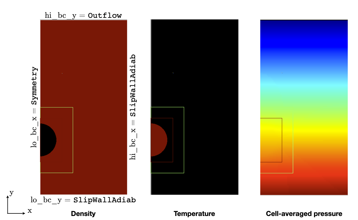
Fig. 9 : Contour plots of density, temperature, cell-averaged pressure after initialization.
The cell-averaged pressure (the perturbational pressure in node-centered in the projection-based scheme employed in PeleLMeX, see Almgren for more details) clearly shows the effect of the gravity field with the presence of an hydrostatic pressure gradient.
Advance the solution
Let’s now advance the solution for 400 steps, using the base grid and 2 AMR level and the default time stepping parameters. To do so, ensure that:
amr.max_step = 400
Additionally, make sure that amr.check_int is set to a positive value to trigger writing a
checkpoint file from which to later restart the simulation. If available, use more than one MPI
rank to run the simulation and redirect the standard output to a log file using:
mpirun -n 4 ./PeleLMeX2d.gnu.MPI.ex input.2d-regt_sym > logInit.dat &
A typical PeleLMeX stdout for a time step now looks like:
====================   NEW TIME STEP   ====================
Est. time step - Conv: 7.249645299e-05, divu: 1e+20
STEP [384] - Time: 0.05931322581, dt 7.249645299e-05
  SDC iter [1]
>> PeleLMeX::Advance() --> Time: 0.2141339779
clearly showing the use of 1 SDC iteration. The first line at each step provides
the time step constraint from the CFL
condition (Conv:) and from the density change condition (divu:).
In the absence of reaction and diffusion, the divu: constraint is irrelevant and set to a
large value.
Visualizing the plt00400 file, we can see that the solution has evolved. The light bubble started rising under the effect of buoyancy, resulting in a shear layer at the interface of between the hot and cold gases. Vorticies appears in the shear layer, wrinking the interface. Smearing of the temperature gradient at the interface is induced by the numerical scheme diffusion, but appearances of local extrema are very limited.
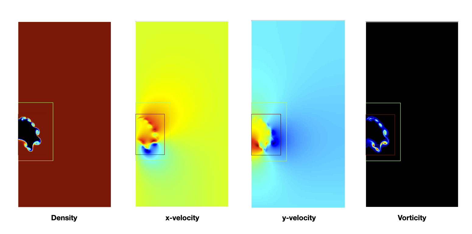
Fig. 10 : Contour plots of density, both velocity components and vorticity after 400 steps.
In order to compare 2D-cartesian and 2D-RZ, you can now start another simulation using input.2d-regt_symRZ. To insure both simulations evolved for the same physical time, set the final time of the 2D-RZ simulation to that of the first run:
amr.max_step = 1000
amr.stop_time = 0.060458236391426
and change the prefix of the plotfile output for clarity:
amr.plot_file = "pltRZ"
then start the 2D-RZ run:
mpirun -n 4 ./PeleLMeX2d.gnu.MPI.ex input.2d-regt_symRZ > logInitRZ.dat &
The 2D-RZ simulation is found to have a smaller time step size resulting from the stronger acceleration of the bubble. Indeed, in the 2D-cartesian case, the hot region is actually an infinitely long cylinder which has inertia larger than that of the bubble effectively represented in the 2D-RZ case.
This is end of the guided section of this tutorial. Interested users can explore the effects of the following parameters on the simulation results since the computational time is minimal:
Spatial resolution: increase the maximum number of AMR levels, ensuring that the simulation final time matches that of the initial run. What is the effect on the rising bubble’s velocity and shape ?
Switch to a mixture composition change instead of a temperature one or reverse the problem by using a bubble temperature lower than that of the ambient air.
Switch to a different advection scheme (see the PeleLMeX controls page for a list of available schemes). What is the effect on the interface wrinkling and smearing ?
If your computational resources allows, build the 3D version of the case and compare the 2D-RZ and 3D results.
In-situ visualization with Ascent
PeleLMeX supports in-situ visualization via Ascent, an open-source many-core capable lightweight in-situ visualization and analysis library developed as part of the Alpine project. Ascent uses Conduit to describe and pass simulation data, and the Viskores library for rendering on both CPU and GPU. Since the solver state is passed directly to Ascent without writing to disk, in-situ rendering eliminates the I/O bottleneck of traditional post-hoc workflows and is well-suited to large-scale GPU runs.
Note
Ascent and Conduit must be built and installed before enabling in-situ
visualization. Refer to the Ascent build documentation and the
Conduit build documentation for
instructions. The build_ascent.sh script provided in the Ascent
repository (scripts/build_ascent/build_ascent.sh) builds both Ascent
and Conduit together and is the recommended approach.
Building with Ascent
Ascent support is enabled at compile time by passing the following flags to
the GNUmake build system (the HotBubble GNUmakefile is unchanged):
make -j8 USE_CUDA=TRUE CUDA_ARCH=89         \
         USE_ASCENT=TRUE                    \
         ASCENT_DIR=/path/to/ascent/install \
         USE_CONDUIT=TRUE                   \
         CONDUIT_DIR=/path/to/conduit/install
Replace /path/to/ascent/install and /path/to/conduit/install with the
paths to your Ascent and Conduit installations. CUDA_ARCH should match your
GPU’s compute capability (e.g., 89 for NVIDIA RTX 40-series, 80 for
A100). Omit the USE_CUDA flags to build a CPU-only Ascent-enabled
executable.
Runtime activation
Ascent is activated at runtime by adding the following to the input file (or passing on the command line):
ascent.plot_int = 10 # call Ascent every 10 time steps
When ascent.plot_int is not set or is negative, Ascent is disabled and
there is no runtime overhead.
Ascent reads a YAML actions file named ascent_actions.yaml from the run
directory automatically. This file describes what to render. A reference file
is provided in the HotBubble case directory:
Exec/RegTests/HotBubble/ascent_actions.yaml
The reference file defines two scenes rendered simultaneously at each in-situ call with no additional solver cost:
-
  action: "add_scenes"
  scenes:
    scene1:
      image_prefix: "hotbubble_temp_%05d"
      plots:
        plt1:
          type: "pseudocolor"
          field: "temp"
    scene2:
      image_prefix: "hotbubble_mesh_%05d"
      plots:
        plt1:
          type: "pseudocolor"
          field: "temp"
        plt2:
          type: "mesh"
scene1 renders the temperature field as a pseudocolor image.
scene2 renders the same temperature field with the AMR mesh overlaid,
clearly showing the block-structured refinement levels that PeleLMeX
automatically generates around the bubble interface.
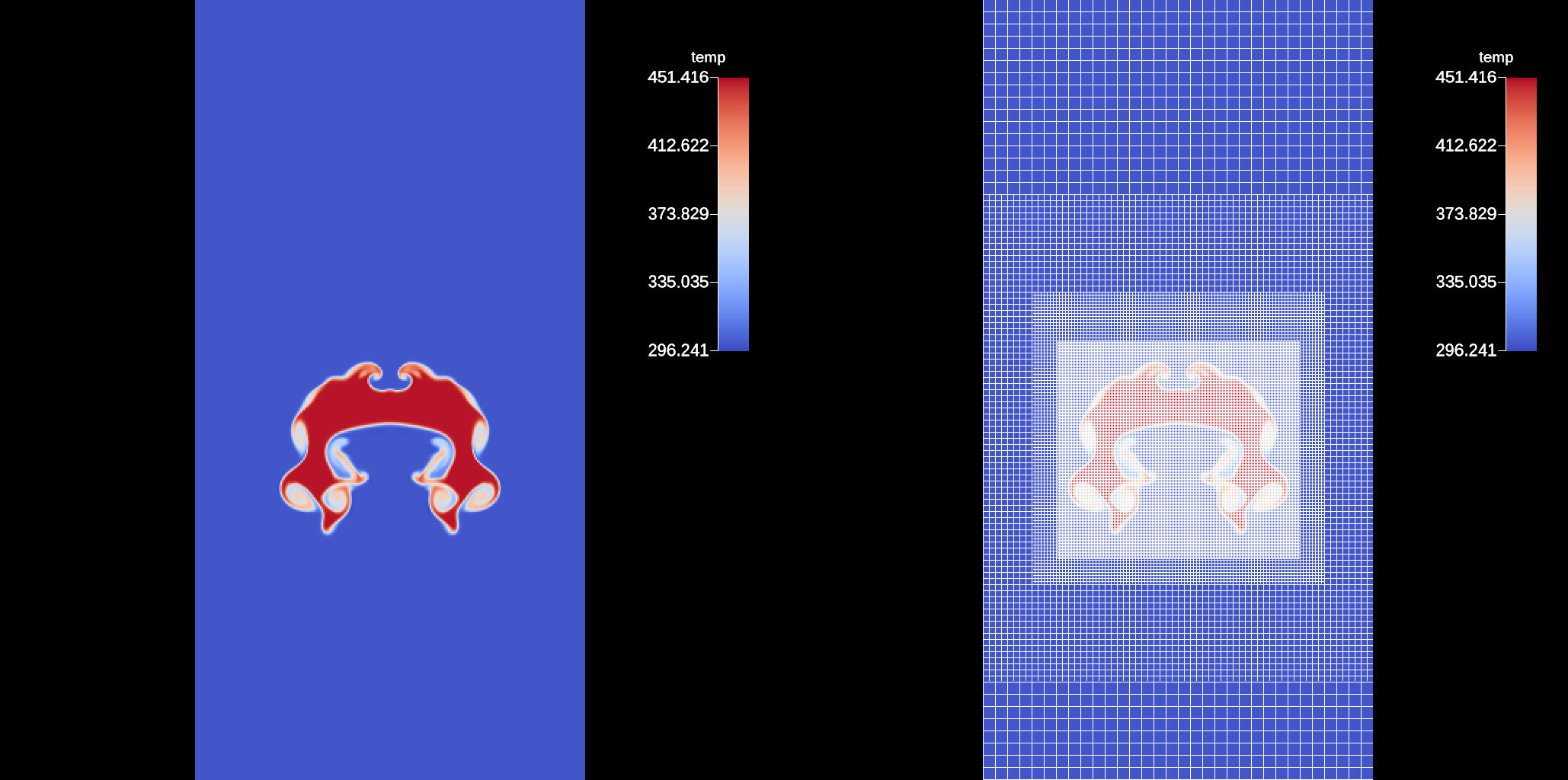
Fig. 11 : Temperature field (left) and temperature with AMR mesh overlay (right) at step 200.
Ascent automatically selects the best available rendering backend — CUDA when available, otherwise OpenMP — based on how it was compiled. No additional configuration is required.
Published fields
The following fields from the PeleLMeX state vector are published to Ascent
at each in-situ call and are available for rendering in ascent_actions.yaml:
x_velocity,y_velocity(z_velocityin 3D)densityrho.Y(<species>)for each species in the mechanism (e.g.rho.Y(N2))rhohtempRhoRT
Example run
To run the HotBubble case with in-situ rendering every 50 steps:
mpirun -n 1 ./PeleLMeX2d.gnu.MPI.CUDA.ex input.2d-regt \
    amr.max_step=400 amr.plot_int=-1 amr.check_int=-1   \
    ascent.plot_int=50
For more information on available Ascent actions (contours, volume rendering, Cinema databases, triggers, etc.), see the Ascent actions documentation.