A simple triple flame
Introduction
Laminar flames have the potential to reveal the fundamental structure of combustion without the added complexities of turbulence. They also aid in our understanding of the more complex turbulent flames. Depending on the fuel involved and the flow configuration, the laminar flames can take on a number of interesting geometries. For example, as practical combustion systems often operate in partially premixed mode, with one or more fuel injections, a wide range of fresh gas compositions can be observed; and these conditions favor the appearance of edge flames, see Fig. 25.

Fig. 25 : Normalized heat release rate (top) and temperature (bottom) contours of two-dimensional (2D) laminar lifted flames of ethylene.
Edge flames are composed of lean and rich premixed flame wings usually surrounding a central anchoring diffusion flame extending from a single point [PCI2007]. Edge flames play an important role in flame stabilization, re-ignition and propagation. Simple fuels can exhibit up to three burning branches while diesel fuel, with a low temperature combustion mode, can exhibit up to 5 branches.
The goal of this TripleFlame tutorial is to setup a simple 2D laminar triple edge flame configuration with PeleLMeX.
This document provides step by step instructions to properly set-up the domain and boundary conditions,
construct an initial solution, and provides guidance on how to monitor and influence the initial transient to reach
a final steady-state solution.
Setting-up your environment
Getting a functioning environment in which to compile and run PeleLMeX is the first step of this tutorial. Follow the steps listed below to get to this point:
The first step is to get PeleLMeX and its dependencies. To do so, use a recursive git clone:
git clone --recursive --shallow-submodules --single-branch https://github.com/AMReX-Combustion/PeleLMeX.git
The
--shallow-submodulesand--single-branchflags are recommended for most users as they substantially reduce the size of the download by skipping extraneous parts of the git history. Developers may wish to omit these flags in order download the complete git history of PeleLMeX and its submodules, though standardgitcommands may also be used after a shallow clone to obtain the skipped portions if needed.Move into the Exec folder containing your tutorial. To do so:
cd PeleLMeX/Exec/RegTests/<CaseName>
where <CaseName> is the name of your tutorial, e.g.
HotBubble,FlameSheet,EB_BackwardStepFlame,EB_FlowPastCylinder, orTripleFlame.
You’re good to go!
Note
The makefile system is set up such that default paths are automatically set to the submodules obtained with the recursive git clone, however advanced users can set their own dependencies in the GNUmakefile for each case by updating the top-most lines as follows:
PELE_HOME     = <path_to_PeleLMeX>
AMREX_HOME        = <path_to_MyAMReX>
AMREX_HYDRO_HOME  = <path_to_MyAMReXHydro>
PELE_PHYSICS_HOME = <path_to_MyPelePhysics>
SUNDIALS_HOME     = <path_to_MySUNDIALS>
or directly through shell environment variables (using bash for instance):
export PELE_HOME=<path_to_PeleLMeX>
export AMREX_HOME=<path_to_MyAMReX>
export AMREX_HYDRO_HOME=<path_to_MyAMReXHydro>
export PELE_PHYSICS_HOME=<path_to_MyPelePhysics>
export SUNDIALS_HOME=<path_to_MySUNDIALS>
Note that using the first option will overwrite any environment variables you might have previously defined when using this GNUmakefile.
Test case and boundary conditions
Direct Numerical Simulations (DNS) are performed on a 2x4 \(cm^2\) 2D computational domain using a 64x128 base grid and up to 4 levels of refinement (although we will start with a lower number of levels). The refinement ratio between each level is set to 2. With 4 levels, this means that the minimum grid size inside the reaction layer will be just below 20 \(μm\). The maximum box size is fixed at 32, and the base (level 0) grid is composed of 8 boxes, as shown in Fig. 26.
Symmetric boundary conditions are used in the transverse (\(x\)) direction, while Inflow (dirichlet)
and Outflow (neumann) boundary conditions are used in the main flow direction (\(y\)). The flow goes
from bottom to top. The specificities of the Inflow boundary condition are explained in hereafter.
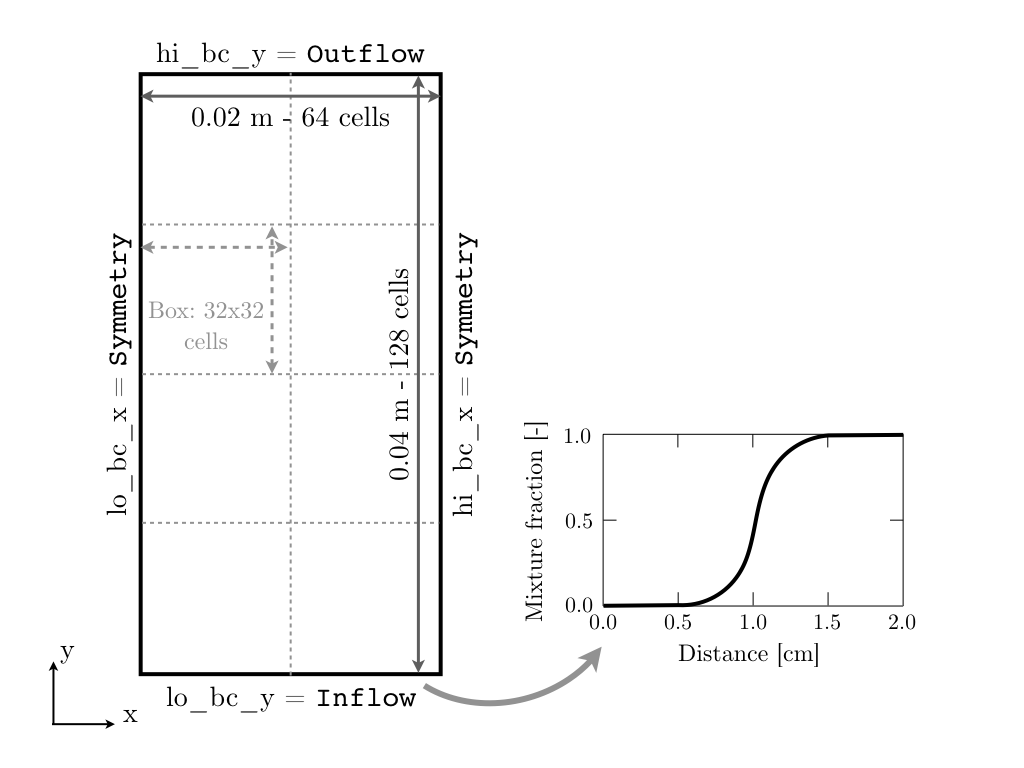
Fig. 26 : Sketch of the computational domain with level 0 box decomposition (left) and input mixture fraction profile (right).
The geometry of the problem is specified in the first block of the input.2d-regt:
#---------------------- DOMAIN DEFINITION ------------------------
geometry.is_periodic = 0 0                # For each dir, 0: non-perio, 1: periodic
geometry.coord_sys   = 0                  # 0 => cart, 1 => RZ
geometry.prob_lo     = 0.0 0.0 0.0        # x_lo y_lo (z_lo)
geometry.prob_hi     = 0.02 0.04 0.0      # x_hi y_hi (z_hi)
The second block determines the boundary conditions. Refer to Fig Fig. 26:
#---------------------- BC FLAGS ---------------------------------
# Interior, Inflow, Outflow, Symmetry,
# SlipWallAdiab, NoSlipWallAdiab, SlipWallIsotherm, NoSlipWallIsotherm
peleLM.lo_bc = Symmetry Inflow            # bc in x_lo y_lo (z_lo)
peleLM.hi_bc = Symmetry Outflow           # bc in x_hi y_hi (z_hi)
The number of levels, refinement ratio between levels, maximum grid size as well as other related refinement parameters are set under the third block :
#---------------------- AMR CONTROL ------------------------------
amr.n_cell          = 64 128              # Level 0 number of cells in each direction
amr.max_level       = 1                   # maximum level number allowed
amr.ref_ratio       = 2 2 2 2             # refinement ratio
amr.regrid_int      = 2                   # how often to regrid
amr.n_error_buf     = 1 1 2 2             # number of buffer cells in error est
amr.grid_eff        = 0.7                 # what constitutes an efficient grid
amr.blocking_factor = 16                  # block factor in grid generation (min box size)
amr.max_grid_size   = 32                  # max box size
Problem specifications
The edge flame is stabilized against an incoming mixing layer with a uniform velocity profile. The mixing layer is prescribed using an hyperbolic tangent of mixture fraction \(z\) between 0 and 1, as can be seen in Fig. 26:
where \(z\) is based on the classical elemental composition [CF1990]:
where \(\beta\) is Bilger’s coupling function, and subscript \(ox\) and \(fu\) correspond to oxidizer and fuel streams respectively.
Specifying dirichlet Inflow conditions in PeleLMeX can seem daunting at first. But it is actually a very
flexible process. We walk the user through the details of it for the Triple Flame case just described. The files involved are:
pelelmex_prob.H, assemble two C++ structsMyProbParmcontains the input variables as well as other variables used in the initialization process, whileMyProblemSpecificFunctionsgathers the functions responsible for generating the initial and boundary conditions (amongst others),initdataandbcnormal.pelelmex_prob.cpp, initialize and provide default values to the entries ofMyProbParmand allow the user to pass run-time value using the AMReX parser (ParmParse). In the present case, the parser will read the parameters in theProblemblock:#---------------------- Problem ---------------------------------- prob.P_mean = 101325.0 prob.T_in = 300.0 prob.V_in = 0.85 prob.Zst = 0.055
Note that in our specific case, we compute the input value of the mass fractions (Y) directly in MyProblemSpecificFunctions::bcnormal,
using the MyProbParm variables. We do not need any additional information, because we hard coded the hyperbolic
tangent profile of \(z\) (see previous formula) and there is a direct relation with the mass fraction profiles.
The interested reader can look at the function set_Y_from_Ksi and set_Y_from_Phi in pelelmex_prob.H.
Looking closely at the MyProbParm struct, we can see that an object specific to
PeleLMeX is present, a FlowControllerData named FCData:
struct MyProbParm::ProbParmDefault
{
    amrex::Real P_mean = 101325.0_rt;
    amrex::Real splitx = 0.0;
    amrex::Real midtanh = 0.001;
    amrex::Real widthtanh = 0.001;
    amrex::Real Zst = 0.05;
    amrex::Real T_in = 300.0;
    amrex::Real V_in = 0.4;

    int bathID{-1};
    int fuelID{-1};
    int oxidID{-1};

    FlowControllerData FCData;
};
This tutorial will use PeleLMeX active control capabilities for which having this object in MyProbParm is necessary (and checked during initialization).
As the simulation proceeds, the data in that container will be updated and used in MyProblemSpecificFunctions::bcnormal to modify the inlet velocity.
Initial solution
An initial field of the main variables is always required to start a simulation. Ideally, you want for this initial solution to approximate the final (steady-state in our case) solution as much as possible. This will speed up the initial transient and avoid many convergence issues. In the present tutorial, an initial solution is constructed by imposing the same inlet hyperbolic tangent of mixture fraction than described in subsection Problem specifications everywhere in the domain, and reconstructing the species mass fraction profiles from it. To ensure ignition of the mixture, a progressively widening Gaussian profile of temperature is added, starting from about 1 cm, and stretching until the outlet of the domain. The initial temperature field is shown in Fig Fig. 27, along with the parameters controlling the shape of the hot spot.
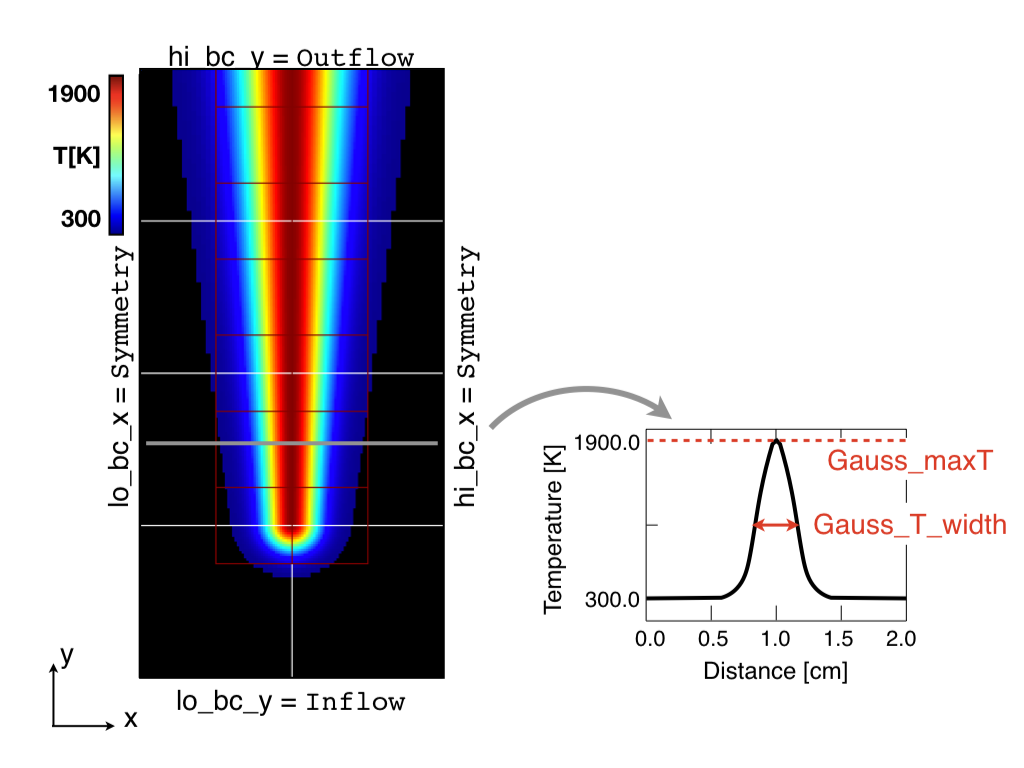
Fig. 27 : Initial temperature field (left) as well as widening gaussian 1D y-profiles (right) and associated parameters. The initial solution contains 2 levels.
This initial solution is constructed via the routine MyProblemSpecificFunctions::initdata(), in the file pelelmex_prob.H. Additional information is provided as comments in this file for the eager reader, but nothing is required from the user at this point.
Numerical scheme
The PeleLM CONTROL block contains a few of the PeleLMeX algorithmic parameters. Many more
unspecified parameters are relying on their default values which can be found in PeleLMeX controls.
Of particular interest are the peleLM.sdc_iterMax parameter controlling the number of
SDC iterations (see The PeleLMeX Model for more details on SDC in PeleLMeX) and the
peleLM.num_init_iter one controlling the number of initial iteration the solver will do
after initialization to obtain a consistent pressure and velocity field.
Building the executable
Now that we have reviewed the basic ingredients required to setup the case, it is time to build the PeleLMeX executable.
Although both GNUmake and CMake are available, it is advised to use GNUmake. The GNUmakefile file provides some compile-time options
regarding the simulation we want to perform.
The first few lines specify the paths towards the source codes of PeleLMeX, AMReX, AMReX-Hydro and PelePhysics, overwriting
any environment variable if necessary, and might have been already updated in Setting-up your environment earlier.
The next few lines specify AMReX compilation options and compiler selection:
# AMREX
DIM             = 2
DEBUG           = FALSE
PRECISION       = DOUBLE
VERBOSE         = FALSE
TINY_PROFILE    = FALSE

# Compilation
COMP            = gnu
USE_MPI         = TRUE
USE_OMP         = FALSE
USE_CUDA        = FALSE
USE_HIP         = FALSE
USE_SYCL        = FALSE
In PeleLMeX, the chemistry model (set of species, their thermodynamic and transport properties as well as the description of their of chemical interactions) is specified at compile time. Chemistry models available in PelePhysics can used in PeleLMeX by specifying the name of the folder in PelePhysics/Mechanisms containing the relevant files, for example:
Chemistry_Model = drm19
Here, the methane kinetic model drm19, containing 21 species is employed. Advanced users may also specify
USE_CUSTOM_CHEMISTRY = TRUE, in which case Chemistry_Model is interpreted as a path and can point to models not included in
PelePhysics by default, though the new model directory must contain valid chemistry model files. The user is referred to
the PelePhysics documentation for a list of available
mechanisms and more information regarding the EOS, chemistry and transport models specified:
Eos_Model       := Fuego
Transport_Model := Simple
Finally, PeleLMeX utilizes the chemical kinetic ODE integrator CVODE. This Third Party Library (TPL) is shipped as a submodule of the PeleLMeX distribution and can be readily installed through the makefile system of PeleLMeX. To do so, type in the following command:
make TPL
Note that the installation of CVODE requires CMake 3.23.1 or higher.
You are now ready to build your first PeleLMeX executable !! Type in:
make -j4
The option here tells make to use up to 4 processors to create the executable (internally, make follows a dependency graph to ensure any required ordering in the build is satisfied). This step should generate the following file (providing that the build configuration you used matches the one above):
PeleLMeX2d.gnu.MPI.ex
You’re good to go !
Initial transient phase
First step: the initial solution
When performing time-dependent numerical simulations, it is good practice to verify the initial solution. To do so,
we will run PeleLMeX to perform the initialization only, to generate an initial plotfile plt00000.
Time-stepping parameters in input.2d-regt are specified in the Time Stepping block:
#---------------------- Time Stepping CONTROL --------------------
amr.max_step = 0                          # Maximum number of time steps
amr.stop_time = 4.00                      # final simulation physical time
amr.cfl = 0.2                             # CFL number for hyperbolic system
amr.dt_shrink = 0.001                     # Scale back initial timestep
amr.dt_change_max = 1.1                   # Maximum dt increase btw successive steps
The maximum number of time steps is set to 0 for now, while the final simulation time is 4.0 s. Note that,
when both max_step and stop_time are specified, the more stringent constraint will control the
termination of the simulation. PeleLMeX solves for the advection, diffusion and reaction processes in time,
but only the advection term is treated explicitly and thus it constrains the maximum time step size
\(dt_{CFL}\). This constraint is formulated with a classical Courant-Friedrich-Levy (CFL) number,
specified via the keyword amr.cfl. Additionally, as it is the case here, the initial solution is often made-up by
the user and local mixture composition and temperature can result in the introduction of unreasonably fast chemical scales.
To ease the numerical integration of this initial transient, the parameter amr.dt_shrink allows to shrink the initial dt
(evaluated from the CFL constraint) by a factor (usually smaller than 1), and let it relax towards \(dt_{CFL}\) at
a rate given by amr.dt_change_max as the simulation proceeds.
Input/output from PeleLMeX are specified in the IO CONTROL block:
#---------------------- IO CONTROL -------------------------------
#amr.restart = chk01000                   # Restart checkpoint file
amr.check_int = 2000                      # Frequency of checkpoint output
amr.plot_int = 20                         # Frequency of pltfile output
amr.derive_plot_vars = avg_pressure mag_vort mass_fractions mixture_fraction progress_variable
The first lines (commented out for now) are only used when restarting a simulation from a checkpoint file and
will be useful later during this tutorial. Information pertaining to the checkpoint and plot_file files name and output
frequency can be specified there (see PeleLMeX controls for a complete list of available keys). PeleLMeX will always
generate an initial plotfile plt00000 if the initialization is properly completed and plotfile IO is triggered,
and a final plotfile at the end of the simulation. It is possible to request including derived variables in the plotfiles
by appending their names to the amr.derive_plot_vars keyword. These variables are derived from the state variables
(velocity, density, temperature, \(\rho Y_k\), \(\rho h\)) which are automatically included in the plotfile.
You finally have all the information necessary to run the first of several steps to generate a steady triple flame. Type in:
./PeleLMeX2d.gnu.MPI.ex input.2d-regt
If you wish to store the standard output of PeleLMeX for later analysis, you can instead use:
./PeleLMeX2d.gnu.MPI.ex input.2d-regt > logCheckInitialSolution.dat &
Whether you have used one or the other command, within 10 s you should obtain a plt00000 file (or even more,
appended with .old*********** if you used both commands). Use Amrvis
to visualize plt00000 and make sure the solution matches the one shown in Fig. Fig. 27.
Running the problem on a coarse grid
As mentioned above, the initial solution is relatively far from the steady-state triple flame we wish to obtain.
An inexpensive and rapid way to transition from the initial solution to an established triple flame is to perform
a coarse (using only 2 AMR levels) simulation using a single SDC iteration for a few initial number of time steps
(here we start with 1000). To do so, update (or verify !) these associated keywords in the input.2d-regt:
#---------------------- AMR CONTROL ------------------------------
...
amr.max_level         = 1                 # maximum level number allowed
...
#---------------------- Time Stepping CONTROL --------------------
...
amr.max_step          = 1000              # maximum number of time steps
...
#---------------------- PeleLM CONTROL ---------------------------
...
peleLM.sdc_iterMax    = 1                 # Number of SDC iterations
To be able to complete this first step relatively quickly, it is advised to run PeleLM using at least 4 MPI processes if possible. It will then take around 10 mn to reach completion. To be able to monitor the simulation while it is running, use the following command:
mpirun -n 4 ./PeleLMeX2d.gnu.MPI.ex input.2d-regt > logCheckInitialTransient.dat &
A plotfile is generated every 20 time steps (as specified via the amr.plot_int keyword in the IO CONTROL block). This will
allow you to visualize and monitor the evolution of the flame. Use the following command to open multiple plotfiles at once
with Amrvis:
amrvis -a plt????0
An animation of the flame evolution during the entire tutorial, including this initial transient, is provided in Fig. 28.
Fig. 28 : Temperature (left) and divu (right) fields from 0 to 2000 time steps (0-?? ms).
Steady-state problem: activating the flame control
The speed of propagation of a triple flame is not easy to determine a-priori. As such it is useful, at least until the flame settles, to have some sort of stabilization mechanism to prevent flame blow-off or flashback. In the present configuration, the position of the flame front can be tracked at each time step (using an isoline of temperature) and the input velocity is adjusted to maintain its location at a fixed distance from the inlet (1 cm in the present case).
The parameters of the active control are listed in AC CONTROL block of input.2d-regt:
#---------------------- AC CONTROL -------------------------------
active_control.on = 1                     # Use AC ?
active_control.use_temp = 1               # Default in fuel mass, rather use iso-T position ?
active_control.temperature = 1400.0       # Value of iso-T ?
active_control.tau = 1.0e-4               # Control tau (should ~ 10 dt)
active_control.height = 0.01              # Where is the flame held ? Default assumes coordinate along Y in 2D or Z in 3D.
active_control.v = 1                      # verbose
active_control.velMax = 2.0               # Optional: limit inlet velocity
active_control.changeMax = 0.1            # Optional: limit inlet velocity changes (absolute m/s)
active_control.flow_dir  = 1              # Optional: flame main direction. Default: AMREX_SPACEDIM-1
active_control.pseudo_gravity = 1         # Optional: add density proportional force to compensate for the acceleration
                                          #           of the gas due to inlet velocity changes
The first keyword activates the active control and the second one specify that the flame will be tracked
based on an iso-line of temperature, the value of which is provided in the third keyword. The following parameters
control the relaxation of the inlet velocity to the steady state velocity of the triple flame. tau is a relaxation time scale,
that should be of the order of ten times the simulation time-step. height is the user-defined location where the
triple flame should settle, changeMax and velMax control the maximum velocity increment and maximum inlet velocity, respectively.
The user is referred to [CAMCS2006] for an overview of the method and corresponding parameters.
The pseudo_gravity triggers a manufactured force added to the momentum equation to compensate for the acceleration of different density gases.
Once these parameters are set, you continue the previous simulation by uncommenting the first line of the IO CONTROL block in the input file:
amr.restart = chk01000 # Restart checkpoint file
On this line, provide the last checkpoint file generated during the first simulation performed for 1000 time steps.
Finally, update the amr.max_step to allow the simulation to proceed further:
#---------------------- Time Stepping CONTROL --------------------
...
amr.max_step          = 2000          # maximum number of time steps
You are now ready launch PeleLMeX again for another 1000 time steps !
mpirun -n 4 ./PeleLMeX2d.gnu.MPI.ex inputs.2d-regt > logCheckControl.dat &
As the simulation proceeds, an ASCII file tracking the flame position and inlet velocity
(as well as other control variables) is generated: AC_History. You can follow the motion of
the flame tip by plotting the seventh column against the first one (flame tip vs. time step count).
If gnuplot is available on your computer, use the following to obtain the graphs of Fig. 29:
gnuplot
plot "AC_History.dat" u 1:7 w lp
plot "AC_History.dat" u 1:3 w lp
exit
The second plot corresponds to the inlet velocity.
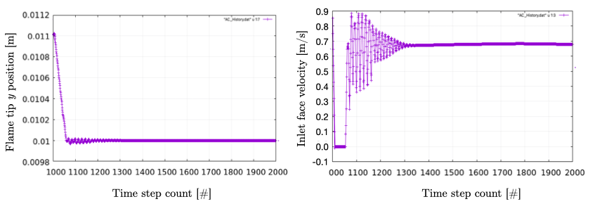
Fig. 29 : Flame tip position (left) and inlet velocity (right) as function of time step count from 1000 to 2000 step using the inlet velocity control.
At this point, you have a stabilized methane/air triple flame and will now use AMR features to improve the quality of your simulation.
Refinement of the computation
Before going further, it is important to look at the results of the current simulation. The left panel of Fig. 30 displays the temperature field, while a zoom-in of the flame edge region colored by several important variables is provided on the right side. Note that DivU, the HeatRelease and the CH4_consumption are good markers of the reaction/diffusion processes in our case. What is striking from these images is the lack of resolution of the triple flame, particularly in the reaction zone. We also clearly see square unsmooth shapes in the field of intermediate species, where Y(HCO) is found to closely match the region of high CH4_consumption while Y(CH3O) is located closer to the cold gases, on the outer layer of the triple flame.
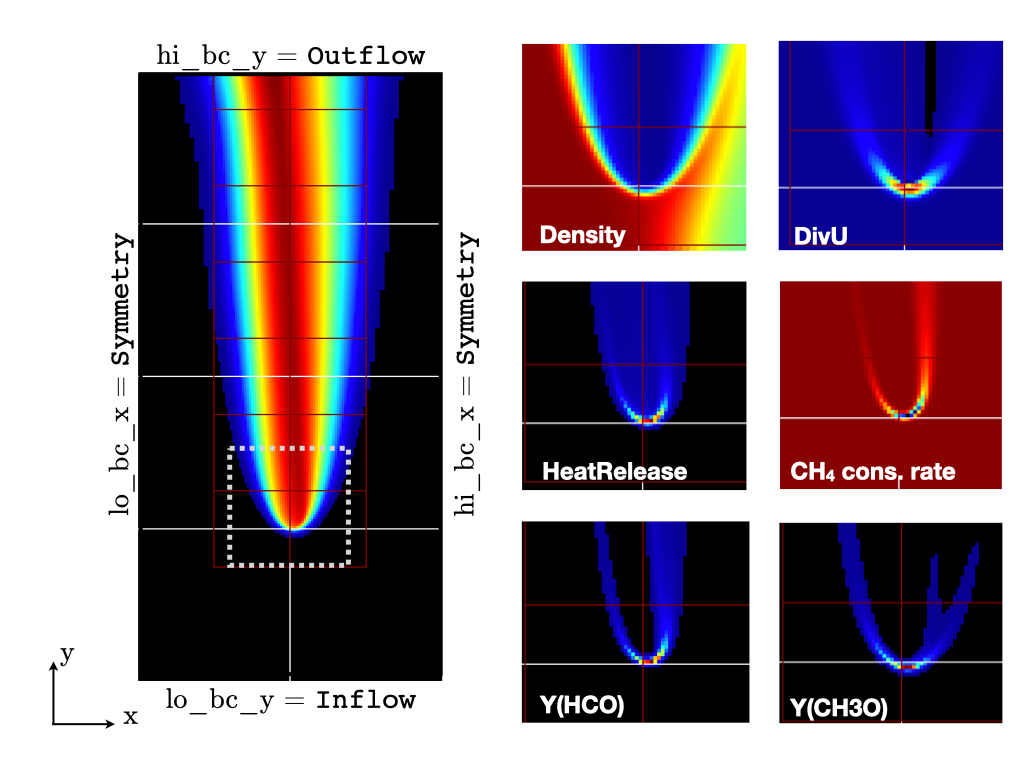
Fig. 30 : Details of the triple flame tip obtained with the initial coarse 2-level mesh.
Our additional level of refinement must specifically target the reactive layer of the flame. As seen from Fig. 30, one can choose from several variables to reach that goal. In the following, we will use the CH3O species as a tracer of the flame position. Start by increasing the number of AMR levels by one in the AMR CONTROL block:
#---------------------- AMR CONTROL ------------------------------
...
amr.max_level       = 2          # maximum level number allowed
Then provide a definition of the new refinement criteria in the Refinement CONTROL block:
#---------------------- Refinement CONTROL------------------------
amr.refinement_indicators = highT gradT flame_tracer   # Declare set of refinement indicators

amr.highT.max_level     = 1
amr.highT.value_greater = 800
amr.highT.field_name    = temp

amr.gradT.max_level                   = 1
amr.gradT.adjacent_difference_greater = 200
amr.gradT.field_name                  = temp

amr.flame_tracer.max_level     = 2
amr.flame_tracer.value_greater = 1.0e-6
amr.flame_tracer.field_name    = Y(CH3O)
The first line simply declares a set of refinement indicators which are subsequently defined. For each indicator,
users can provide a limit up to which AMR level this indicator will be used to refine. Then there are multiple possibilities
to specify the actual criterion: value_greater, value_less, vorticity_greater or adjacent_difference_greater.
In each case, the user specify a threshold value and the name of variable on which it applies (except for the vorticity_greater).
In the example above, the grid is refined up to level 1 at the location wheres the temperature is above 800 K or where the temperature
difference between adjacent cells exceed 200 K. These two criteria were used up to that point. The last indicator will now enable
to add level 2 grid patches at location where the flame tracer (Y(CH3O)) is above 1.0e-6.
With these new parameters, update the checkpoint file from which to restart:
amr.restart = chk02000 # Restart checkpoint file
and increase the amr.max_step to 2500 and start the simulation again !
mpirun -n 4 ./PeleLMeX2d.gnu.MPI.ex input.2d-regt > log3Levels.dat &
Visualization of the 3-levels simulation results indicates that the flame front is now better represented on the fine grid,
but there are still only a couple of cells across the flame front thickness. The flame tip velocity, captured in the AC_history, also
exhibits a significant change with the addition of the third level (even past the initial transient). In the present case,
the flame tip velocity is our main quantity of interest and we will now add another refinement level to ensure that this quantity
is fairly well captured. We will use the same refinement indicators and simply update the amr.max_level as well as the level
at which each refinement criteria is used:
amr.max_level         = 3          # maximum level number allowed

...

amr.restart           = chk02300 # Restart from checkpoint ?

...

amr.gradT.max_level   = 2

...

amr.flame_tracer.max_level  = 3
and increase the amr.max_step to 3000. Within PeleLMeX non-subcycling time advance, the step size is decreasing as we increase the number of AMR
levels. We started with a rather small CFL number of 0.2 to avoid numerical issues associated with coarse simulations and large time step size
(see Backward facing step anchored premixed flame more a practical example of integration failure). Additionally, as our step size decreases, the tau parameter of the
active control becomes comparatively larger, resulting in slower response of the adapted inlet velocity to flame position changes. Let’s increase the
CFL number of 0.3, reduce tau and add a second SDC iteration to tighten the coupling between the various processes:
peleLM.sdc_iterMax = 2

...

amr.cfl = 0.3

...

active_control.tau = 1.0e-4            # Control tau (should ~ 10 dt)
Let’s start the simulation again !
mpirun -n 4 ./PeleLM2d.gnu.MPI.ex inputs.2d-regt > log4Levels.dat &
Figure Fig. 31 shows the entire history of the inlet velocity starting when the AC was activated (1000th time step). We can see that every change in the numerical setup induced a slight change in the triple flame propagation velocity, eventually leading to a nearly constant value, sufficient for the purpose of this tutorial.
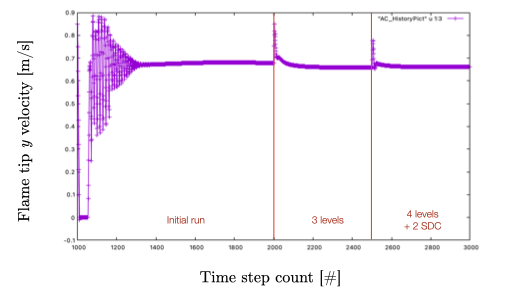
Fig. 31 : Inlet velocity history during the successive simulations performed during this tutorial.
At this point, the simulation is considered complete.
Chung, Stabilization, propagation and instability of tribrachial triple flames, Proceedings of the Combustion Institute 31 (2007) 877–892
Bilger, S. Starner, R. Kee, On reduced mechanisms for methane-air combustion in nonpremixed flames, Combustion and Flames 80 (1990) 135-149
Bell, M. Day, J. Grcar, M. Lijewski, Active Control for Statistically Stationary Turbulent PremixedFlame Simulations, Communications in Applied Mathematics and Computational Science 1 (2006) 29-51