Premixed flame sheet with harmonic perturbations

Introduction

PeleLMeX primary objective is to enable simulation of reactive flows on platforms ranging from small personal computer to Exascale supercomputer. This short FlameSheet tutorial describes the case of a 2D laminar methane/hydrogen/air premixed flame, perturbed using harmonic fluctuations on the initial conditions.

The goal of this tutorial is to demonstrate PeleLMeX basic controls when dealing with reactive simulations. This document provides step by step instructions reviewing how to set-up the domain and boundary conditions, and how to construct an initial solution.

Setting-up your environment

Getting a functioning environment in which to compile and run PeleLMeX is the first step of this tutorial. Follow the steps listed below to get to this point:

The first step is to get PeleLMeX and its dependencies. To do so, use a recursive git clone:
```
git clone --recursive --shallow-submodules --single-branch https://github.com/AMReX-Combustion/PeleLMeX.git
```
The --shallow-submodules and --single-branch flags are recommended for most users as they substantially reduce the size of the download by skipping extraneous parts of the git history. Developers may wish to omit these flags in order download the complete git history of PeleLMeX and its submodules, though standard git commands may also be used after a shallow clone to obtain the skipped portions if needed.
Move into the Exec folder containing your tutorial. To do so:
```
cd PeleLMeX/Exec/RegTests/<CaseName>
```
where <CaseName> is the name of your tutorial, e.g. HotBubble, FlameSheet, EB_BackwardStepFlame, EB_FlowPastCylinder, or TripleFlame.

You’re good to go!

Note

The makefile system is set up such that default paths are automatically set to the submodules obtained with the recursive git clone, however advanced users can set their own dependencies in the GNUmakefile for each case by updating the top-most lines as follows:

PELE_HOME     = <path_to_PeleLMeX>
AMREX_HOME        = <path_to_MyAMReX>
AMREX_HYDRO_HOME  = <path_to_MyAMReXHydro>
PELE_PHYSICS_HOME = <path_to_MyPelePhysics>
SUNDIALS_HOME     = <path_to_MySUNDIALS>

or directly through shell environment variables (using bash for instance):

export PELE_HOME=<path_to_PeleLMeX>
export AMREX_HOME=<path_to_MyAMReX>
export AMREX_HYDRO_HOME=<path_to_MyAMReXHydro>
export PELE_PHYSICS_HOME=<path_to_MyPelePhysics>
export SUNDIALS_HOME=<path_to_MySUNDIALS>

Note that using the first option will overwrite any environment variables you might have previously defined when using this GNUmakefile.

Case setup

A PeleLMeX case folder generally contains a minimal set of files to enable compilation, provide user-defined functions defining initial and boundary conditions, input file(s) and any additional files necessary for the simulation (solution of a Cantera 1D flame for instance).

The following three files in particular are necessary:

pelelmex_prob_parm.H
pelelmex_prob.H
pelelmex_prob.cpp

The first file provides a C++ struct ProbParm containing the set of user-defined variables used during the simulation (value of inlet temperature, amplitude of the initial perturbation, …). The .cpp file uses AMReX ParmParse to read these run-time parameter and initialize the ProbParm container values. Finally, pelelmex_prob.H provides C++ kernels for the initial and boundary conditions and will be detailed later in this tutorial.

The following review the content of the various files required for the flame sheet test case. User keys listed in the input.2d-regt file are reviewed and linked to the specific aspects of the simulation setup. To get additional information about the keywords discussed, the reader is referred to PeleLMeX controls.

Geometry, grid and boundary conditions

This Direct Numerical Simulations (DNS) is performed on a 0.016x0.032 \(m^2\) 2D computational domain, with the bottom left corner located at (0.0:0.0) and the top right corner at (0.016:0.032). Periodic boundary conditions are used in the transverse (\(x\)) direction, while Inflow (dirichlet) and Outflow (0-neumann) boundary are used in the main flow direction (\(y\)). The flow goes from bottom to top. Finally a Cartesian coordinate system is used here. All of the above information is provided in the first two blocks of the input file:

#---------------------- DOMAIN DEFINITION -------------------------
geometry.is_periodic = 1 0             # Periodicity in each direction: 0 => no, 1 => yes
geometry.coord_sys   = 0               # 0 => cart, 1 => RZ
geometry.prob_lo     = 0.0   0.0       # x_lo y_lo
geometry.prob_hi     = 0.016 0.032     # x_hi y_hi

#---------------------- BC FLAGS ----------------------------------
# Interior, Inflow, Outflow, Symmetry,
# SlipWallAdiab, NoSlipWallAdiab, SlipWallIsotherm, NoSlipWallIsotherm
peleLM.lo_bc = Interior Inflow         # bc in x_lo y_lo (z_lo)
peleLM.hi_bc = Interior Outflow        # bc in x_hi y_hi (z_hi)

Note

Note that Interior BC must be imposed in the direction specified as periodic with geometry.is_periodic.

The base grid is decomposed into a 32x64 cells array, and initially 2 levels of refinement are used. When running serial, a single box is used on the base level as the amr.max_grid_size exceeds the number of cells in each direction. When running parallel, the base grid will be chopped into smaller boxes in the limit that no box smaller than the amr.blocking_factor can be created (16 \(^2\) here).

The refinement ratio between each level is set to 2 and PeleLMeX currently does not support refinement ratio of 4. Regrid operation will be performed every 5 steps. amr.n_error_buf specifies, for each level, the number of buffer cells used around the cell tagged for refinement, while amr.grid_eff describes the grid efficiency, i.e. how much of the new grid contains tagged cells. Higher values lead to tighter grids around the tagged cells.

All of those parameters are specified in the AMR CONTROL block:

#------------------------- AMR CONTROL ----------------------------
amr.n_cell          = 32 64            # Level 0 number of cells in each direction
amr.max_level       = 2                # maximum level number allowed
amr.ref_ratio       = 2 2 2 2          # refinement ratio
amr.regrid_int      = 5                # how often to regrid
amr.n_error_buf     = 1 1 2 2          # number of buffer cells in error est
amr.grid_eff        = 0.7              # what constitutes an efficient grid
amr.blocking_factor = 16               # block factor in grid generation
amr.max_grid_size   = 256              # maximum box size

Problem specifications

The problem setup is mostly contained in the three C++ source/header files mentioned above. Looking into pelelmex_prob_parm.H first, we can see the set of parameters that will be used to specify the initial and boundary conditions:

struct ProbParm
{
   amrex::Real P_mean   = 101325.0_rt;
   amrex::Real standoff = 0.0_rt;
   amrex::Real pertmag  = 0.0004_rt;
   amrex::Real pertlength  = 0.008_rt;
};

Because initial and boundary conditions for this case are mostly extracted from a 1D freely propagating premixed flame solution obtained with Cantera, only a handful of parameters need to be specified. The standoff parameter controls the position of the interpolated Cantera solution on the PeleLMeX domain while pertmag and pertlength control the amplitude and transerve length of the harmonic perturbations, respectively. Default values are provided for all the parameter. Note that the domain transverse size (the \(x\) length here) must be a multiple of the pertlength in order to ensure periodicity of the initial solution.

Note

The P_mean parameters, providing the initial thermodynamic pressure, is always needed in the ProbParm struct.

Looking now into pelelmex_prob.cpp, we can see how the developer can provide access to the ProbParm parameters to overwrite the default values using AMReX’s ParmParse:

void PeleLM::readProbParm()
{
   amrex::ParmParse pp("prob");

   std::string type;
   pp.query("P_mean",   PeleLM::prob_parm->P_mean);
   pp.query("standoff", PeleLM::prob_parm->standoff);
   pp.query("pertmag",  PeleLM::prob_parm->pertmag);
   pp.query("pertlength",  PeleLM::prob_parm->pertlength);

   PeleLM::pmf_data.initialize();
}

The PeleLMeX has its own ProbParm instance, the values of which are set by the query function calls. Note that because a query function is employed, the solver will use the default values of the ProbParm parameters if they are not provided in the input file. Use a pp.get to throw an error if overwriting the default value is desirable (see AMReX’s ParmParse documentation for more information). Users can now add the corresponding keys to their input file:

prob.P_mean = 101325.0
prob.standoff = -.023
prob.pertmag = 0.00045
prob.pertlength = 0.016

Additionally, the readProbParm() function initialize another data structure designed to handle the Cantera solution (not detailed here). When this function is called, users must provide the path to the Cantera solution stored as an ASCII file in the input file:

pmf.datafile = "drm19_pmf.dat"

Finally, pelelmex_prob.H defines the two functions effectively filling the initial solution and boundary conditions: pelelmex_initdata and bcnormal. The arguments of the pelelmex_initdata function are as follows:

int i, int j, int k, : indices of the current grid cell the function is called to fill
int /*is_incompressible*/, : flag indicating if PeleLMeX is running a pure incompressible case
amrex::Array4<amrex::Real> const& state, : a lightweight array structure enabling access to the grid state data
amrex::Array4<amrex::Real> const& /*aux*/, : similar array structure but for the auxiliaries data
amrex::GeometryData const& geomdata, : an AMReX object containing geometrical data of the current level
ProbParm const& prob_parm, : the ProbParm struct
pele::physics::PMF::PmfData::DataContainer const * pmf_data : the Cantera solution data struct

The reader is encouraged to look into the body of the pelelmex_initdata function for more details, a skeletal version of the function reads:

Compute the coordinate of the cell center using the cell indices and the geomdata.
Compute the harmonic perturbation.
Using standoff and the perturbation, use the PMF function to get cell-average temperature, mole fractions and velocity from the Cantera solution.
Use the data from the PMF to set the state array: velocities, density, rhoYs, rhoH and temperature. Relying on EOS calls and using ProbParm::P_mean.

Some of the arguments of the bcnormal should now be familiar. The coordinates of the cell where the function is called are now directly passed into the function and the outgoing state vector is now s_ext. The idir and sgn ints can be used to easily determine on which domain face the function in called. Once again, the state vector is extracted from the PMF function to match the operating conditions of the Cantera flame. This function is only called in the direction/orientation where a Dirichlet boundary condition is imposed, i.e. the \(y\)-low domain face here since the transverse direction is periodic and the outflow is an homogeneous Neumann for the state components.

A last function, zero_visc, is included in pelelmex_prob.H but is not used in the present case.

Numerical parameters

The PeleLMeX CONTROL block contains a few of the PeleLMeX algorithmic parameters. Many more unspecified parameters are relying on their default values which can be found in PeleLMeX controls. Of particular interest are the peleLM.sdc_iterMax parameter controlling the number of SDC iterations (see The PeleLMeX Model for more details on SDC in PeleLMeX) and the peleLM.num_init_iter one controlling the number of initial iteration the solver will do after initialization to obtain a consistent pressure and velocity field.

Building the executable

Now that we have reviewed the basic ingredients required to setup the FlameSheet case, it is time to build the PeleLMeX executable. Although both GNUmake and CMake are available, it is advised to use GNUmake. The GNUmakefile file provides some compile-time options regarding the simulation we want to perform. The first few lines specify the paths towards the source codes of PeleLMeX, AMReX, AMReX-Hydro and PelePhysics, overwriting any environment variable if necessary, and might have been already updated in Setting-up your environment earlier.

The next few lines specify AMReX compilation options and compiler selection:

# AMREX
DIM             = 2
DEBUG           = FALSE
PRECISION       = DOUBLE
VERBOSE         = FALSE
TINY_PROFILE    = FALSE

# Compilation
COMP            = gnu
USE_MPI         = TRUE
USE_OMP         = FALSE
USE_CUDA        = FALSE
USE_HIP         = FALSE
USE_SYCL        = FALSE

It allows users to specify the number of spatial dimensions (2D), trigger debug compilation and other AMReX options. The compiler (gnu) and the parallelism paradigm (in the present case only MPI is used) are then selected. If MPI is not available on your platform, please set USE_MPI = FALSE. Note that on OSX platform, one should update the compiler to llvm.

In PeleLMeX, the chemistry model (set of species, their thermodynamic and transport properties as well as the description of their of chemical interactions) is specified at compile time. Chemistry models available in PelePhysics can used in PeleLMeX by specifying the name of the folder in PelePhysics/Mechanisms containing the relevant files, for example:

Chemistry_Model = drm19

Here, the model drm19, contains 21 species and describe the chemical decomposition of methane. The user is referred to the PelePhysics documentation for a list of available mechanisms and more information regarding the EOS, chemistry and transport models specified:

Eos_Model       := Fuego
Transport_Model := Simple

Note that the Chemistry_Model must be similar to the one used to generate the Cantera solution.

Finally, PeleLMeX utilizes the chemical kinetic ODE integrator CVODE. This Third Party Library (TPL) is shipped as a submodule of the PeleLMeX distribution and can be readily installed through the makefile system of PeleLMeX. To do so, type in the following command:

make -j4 TPL

Note that the installation of CVODE requires CMake 3.23.1 or higher.

You are now ready to build your first PeleLMeX executable !! Type in:

make -j4

The option here tells make to use up to 4 processors to create the executable (internally, make follows a dependency graph to ensure any required ordering in the build is satisfied). This step should generate the following file (providing that the build configuration you used matches the one above):

PeleLMeX2d.gnu.MPI.ex

You’re good to go!

Checking the initial conditions

As a first step, we will run the simulation performing only the initialization and visualize the initial condition, while varying some of the problem parameters. To do so, we need to update the time stepping block to specify the number of time steps.

Open the input.2d-regt with your favorite editor and update the following parameters

#---------------------- Time Stepping CONTROL --------------------
amr.max_step      = 0             # Maximum number of time steps
amr.stop_time     = 0.025         # final physical time
amr.max_wall_time = 0.1           # Maximum simulation run time
amr.cfl           = 0.5           # cfl number for hyperbolic system
amr.dt_shrink     = 0.0001        # scale back initial timestep
amr.dt_change_max = 1.1           # Maximum dt increase btw successive steps

We’ve specified three condition upon which PeleLMeX will end the simulation: a maximum number of time steps, a maximum physical simulation time and a maximum wallclock time. As soon as one of these condition is met, the code will exit. The time step size is based on a hydrodynamic CFL set here at 0.5, but this estimated value is multiplied by amr.dt_shrink upon initialization to more smoothly eliminate any numerical noise arising from the state vector initial solution. The step size then relax to the CFL-constrained dt at a rate controlled by amr.dt_change_max.

We’ve set the maximum number of steps to 0 such the solver will exit after the initial solution is obtained. Let’s run the simulation with the default problem parameter listed in the input file. To do so, use:

./PeleLMeX2d.gnu.MPI.ex input.2d-regt

A number of information are printed to the screen:

AMReX/SUNDIALs initialization along with the git hashes of the various subrepositories
A summary of the PeleLMeX state components
PeleLMeX structs initialization: transport, reactor, PMF Cantera structure, AMR hierarchy, …
Initial projection and initial iterations.
Saving the initial solution to plt00000 file.

Use Amrvis, Paraview or yt to visualize the plot file. Using Amrvis, the solution should look similar to Fig. 8.

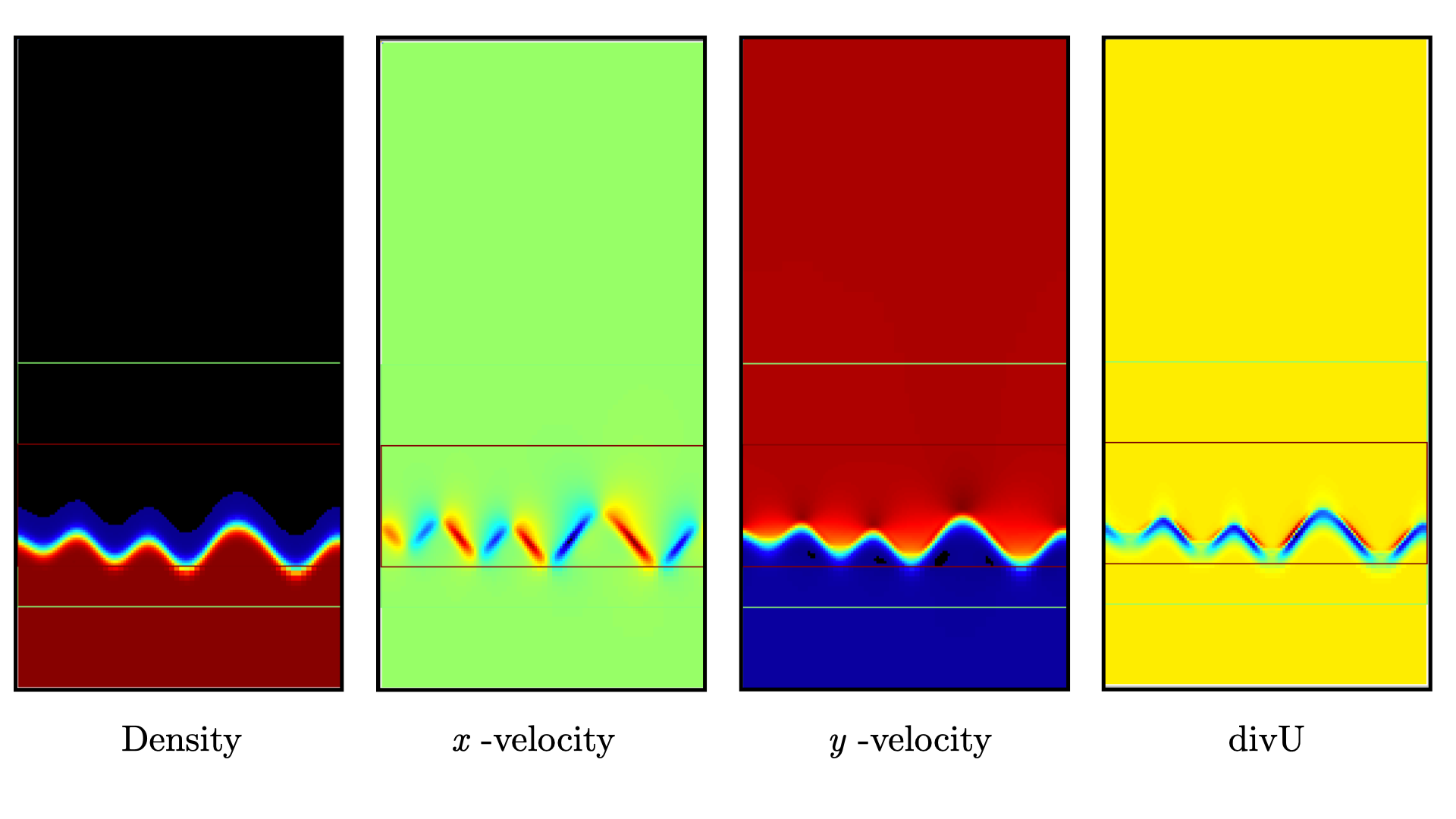
_images/FS_InitSolDefault.png — Fig. 8 : Contour plots of density, velocity components and velocity divergence constraint after initialization.

It is interesting to note that the initial solution has a transverse velocity component even though only the axial velocity was extracted from a 1D Cantera solution to initialize the solution in the pelelmex_initdata function. This is because PeleLMeX performs an initial projection (more than one actually). At this point, the divU constraint is mostly negative, which is counter-intuitive for a flame, but this is the consequence of the initialization process and the solution will rapidly relax to adapt to the PeleLMeX grid.

Let’s now play with the problem parameters to see how the initial solution changes. For instance, decrease the amplitude of the perturbation, change the standoff parameter or deactivate the initial projection by adding peleLM.do_init_proj=0 to the PeleLMeX CONTROL block. Examples of the initial solution varying these parameters are displayed in Fig. 9.

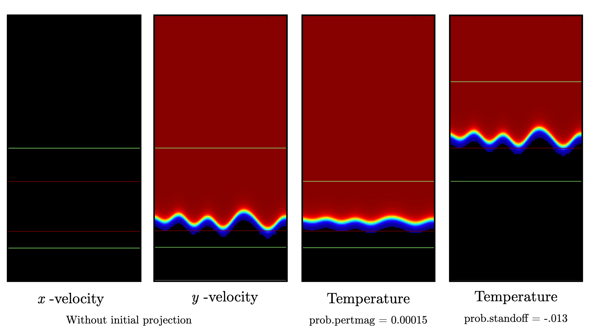
_images/FS_InitSolTweaks.png — Fig. 9 : Contour plots of velocity components without initial projection and temperature using tweaked problem parameter.

Advance the solution

So far, we haven’t advanced the solution at all. Restore the problem parameters to their initial values, re-activate the initial projection and let’s now run the simulation for 50 steps and save a checkpoint file from which to restart from. To do so, ensure that:

amr.max_step = 50

and uncomment the following line to require writing checkpoint files:

amr.check_int = 2000

As soon as this last key is specified, PeleLMeX will write an initial and final checkpoint file. Note that checkpoint file and plotfile store different data. A checkpoint file will store all the necessary state data to enable a continuous restart of the simulation, i.e. the solution after 50 steps is exactly the same as the one obtained running 25 steps first, then restarting for another 25 steps. A plotfile will not necessarily contains the entire state and also includes a number of derived variables of interest to analyse the simulation. The content of a plotfile can be controlled by users using:

amr.derive_plot_vars = avg_pressure mag_vort mass_fractions mixture_fraction progress_variable

Here we require the cell-averaged pressure, the vorticity, species mass fraction (remember that PeleLMeX state contains rhoYs not Ys), mixture fraction and progress variable to be added to the plotfile. For a complete list of PeleLMeX available derived, see the adequate section in PeleLMeX controls.

Additionally, increase PeleLMeX verbose in order to better see the various steps of the algorithm:

peleLM.v = 3

And start the simulation from the beginning again:

./PeleLMeX2d.gnu.MPI.ex input.2d-regt

Using a single processor, it takes about one minute to complete the 50 time steps. A typical PeleLMeX stdout for a time step now looks like:

==============================================================================
Est. time step - Conv: 1.794426504e-05, divu: 0.0002454786986
STEP [10] - Time: 1.892958943e-09, dt 3.080703507e-10
  SDC iter [1]
  - oneSDC()::MACProjection()   --> Time: 0.017529
  - oneSDC()::ScalarAdvection() --> Time: 0.027038
  - oneSDC()::ScalarDiffusion() --> Time: 0.104103
  - oneSDC()::ScalarReaction()  --> Time: 0.220751
  SDC iter [2]
  - oneSDC()::Update t^{n+1,k}  --> Time: 0.103966
  - oneSDC()::MACProjection()   --> Time: 0.012029
  - oneSDC()::ScalarAdvection() --> Time: 0.027831
  - oneSDC()::ScalarDiffusion() --> Time: 0.082195
  - oneSDC()::ScalarReaction()  --> Time: 0.236054
  - Advance()::VelocityAdvance  --> Time: 0.04529
>> PeleLM::Advance() --> Time: 1.07867

clearly showing the use of 2 SDC iterations and the time spent performing projection, computing scalar advection, diffusion and reaction, and finally performing the velocity advance. The reader is referred to The PeleLMeX Model for a detailed description of all of these steps.

The first line at each step provide the time step constraint from the CFL condition (Conv:) and from the density change condition (divu:). Since an initial dt_shrink was applied upon initialization, the current step is much smaller than the CFL but progressively increases over the course of the 50 steps.

Visualizing the plt00050 file, we can see that the solution has not changed much from the initial solution at this point (only a fraction of a microsecond runtime has been reached). It is still interesting to look more closely at divU, FunctCall, the thermodynamic pressure and an intermediate species such as CH3 in Fig. 10.

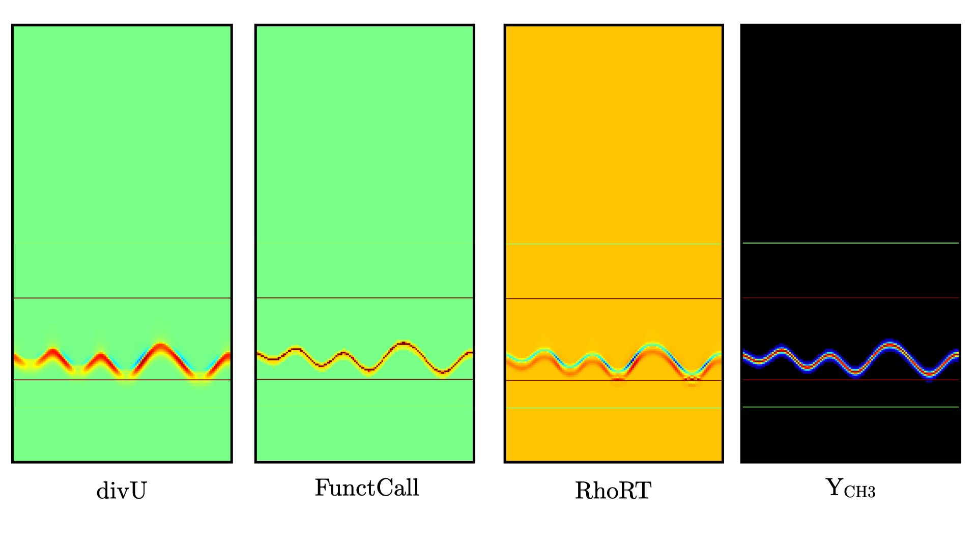
_images/FS_50steps.png — Fig. 10 : Contour plots of divU, FunctCall, thermodynamic pressure and CH3 mass fraction after 50 steps.

The divU is now mostly positive, consistent with the thermal expansion occurring across a flame front. The FunctCall is the number of calls to the chemical right-hand-side function used in the chemical integrator CVODE. Higher values are indicative of locally stiffer chemical ODE system, concentrated in the reactive layer of the flame. The RhoRT variable is the thermodynamic pressure: within PeleLMeX low Mach number approach, this should be perfectly uniform in space. However to conserve mass and enthalpy, the PeleLMeX algorithm allows for small deviation from this constraint. In the current case, deviation do not extend 0.0001 Pa, but larger deviations (> 100-1000 Pa) can be indicative that more SDC iterations are necessary or that the time step size is too large. Finally, we can see from looking at the CH3 mass fraction that the current spatial resolution is barely able to capture the internal flame structure.

Let’s now continue the simulation, restarting from the chk00050 file and adding another level of refinement. To do so, uncomment the following line:

amr.restart = chk00050

Increase the max_step to 120 and increase the maximum level to 3:

amr.max_level       = 3

And restart the simulation, now using more than one MPI ramk if possible:

mpirun -n 2 ./PeleLMeX2d.gnu.MPI.ex input.2d-regt

Because the step size keeps increasing, the physical simulation time after 120 steps is now around 0.1 ms. Upon restarting the simulation, a third refinement level was added as requested:

====================   NEW TIME STEP   ====================
Regridding...
Remaking level 1
with 4096 cells, over 50% of the domain
Remaking level 2
with 8192 cells, over 25% of the domain
Making new level 3 from coarse
with 20480 cells, over 15.625% of the domain
Resetting fine-covered cells mask
Update chemistry typical values

The finest level contains more cells than the sum of all the other levels while only occupying about 15% of the domain, showing how AMR is able to provide local refinement only around the location of interest. In the present case, refinement is triggered by a threshold value on the H species. This option is specified in the input file using:

#---------------------- Refinement CONTROL------------------------
amr.refinement_indicators = yH
amr.yH.max_level     = 3
amr.yH.value_greater = 1.0e-6
amr.yH.field_name    = Y(H)

Users can freely add additional refinement indicator to trigger refinement is other part of the domain. Note also that if we were to add another level of refinement, the amr.yH.max_level should be increased in order to trigger refinement up to level 4 with this criteria.

Fig. 11 shows the same variables as Fig. 10. divU is now almost entirely positive and shows lower values near the tip of the flame cusps as expected from a lean methane/air flame (the amount of hydrogen in the inlet stream is small). The scale of FunctCall increased from a maximum of 12 to 35, indicating that as the step size is increased, CVODE requires more RHS call to integrate the chemical system. Similarly, RhoRT is found to deviate more from the 1 Atm uniform value, up to 25 Pa. also as a consequence of the large time step size (about 10 \(\mu s\) by the end of the simulation). Finally, the CH3 mass fraction field show that the intermediate species is now resolved on more than a single cell (but more refienement would be necessary if this species was of special interest).

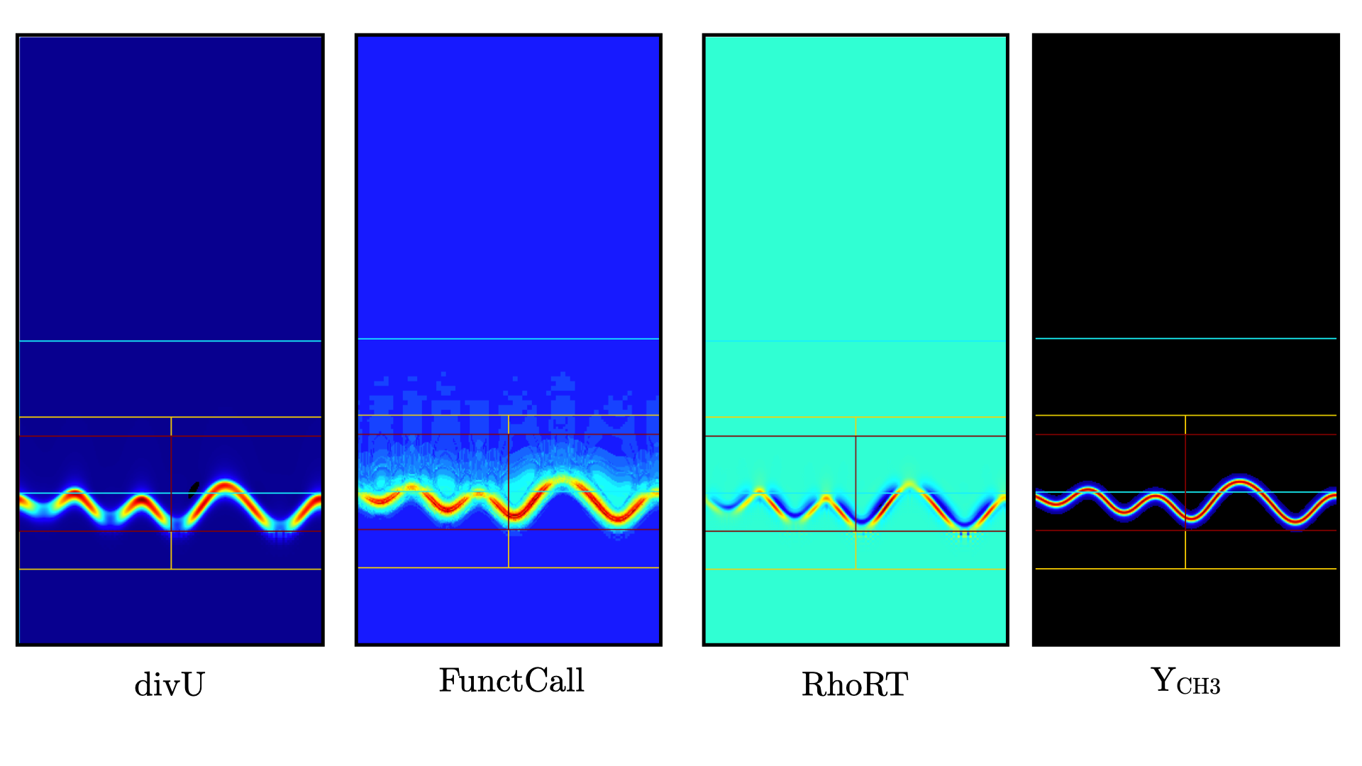
_images/FS_120steps.png — Fig. 11 : Contour plots of divU, FunctCall, thermodynamic pressure and CH3 mass fraction after 120 steps.

This is the end of this short tutorial introducing the basics of reactive flow simulations with PeleLMeX. More advanced aspects of the code are described in other tutorials and readers can peruse the numerous case folders available in Exec to find example in order to set their own case.