Converging Nozzle Case
Case description
This is a round inviscid converging nozzle case that can be compared against analytical relationships for quasi-one dimensional isentropic compressible flow. The nozzle is set up with an inlet Mach number of 0.22, and area ratio of 2, and an outlet pressure of 1 bar. The case uses the gamma law equation of state with \(\gamma=1.4\). Rudimentary sponge zones are added at the inlet and outlet to absorb spurious reflected waves.
Property Comparisons to Quasi-1D Flow
Here, we compare property profiles extracted from the centerline of the nozzle to analytical profiles derived from the quasi-1D flow assumption. The relationship
is used to determine the analytical Mach number, and then this is converted to a pressure ratio using
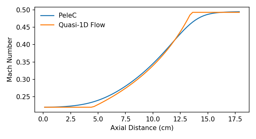
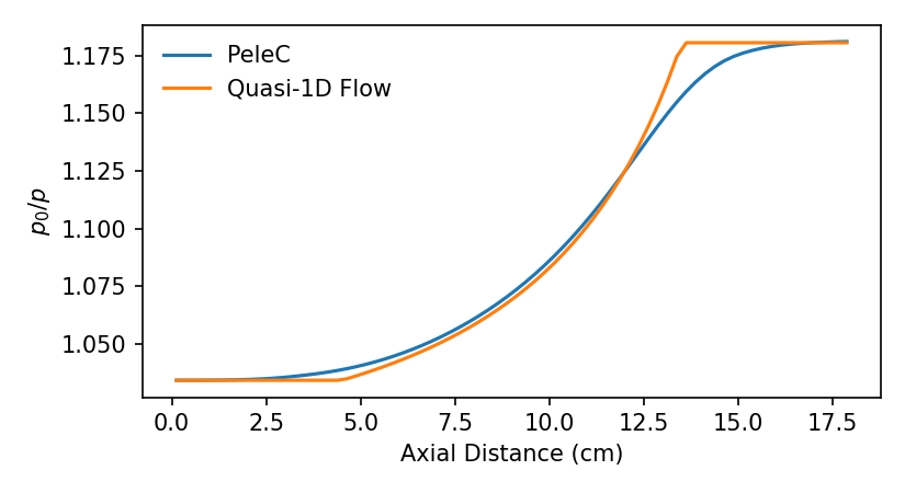
There is some discrepancy between the 3D simulation and the analytical quasi-1D profiles, especially near the beginning and end of the converging section of the nozzle, which is to be expected due to the sharp change in flow direction at these locations for the 3D simulation. The key result is that the inlet and outlet conditions match the theoretical predictions.
Effect of Boundary Conditions
Here, we compare three potential subsonic inlet/outlet boundary condition settings. The first is the naive choice where all flow variables are fixed at the inlet and first-order extrapolation is used for all flow variables at the exit. The second also uses first-order extrapolation at the outlet, but for the inlet pressure is taken from the interior cells and all other flow variables are fixed. The final strategy uses this specification at the inlet and at the outlet applies a characteristic-based extrapolation that allows the exterior pressure to be specified. This outlet specification comes from Whitfield and Janus (Three-Dimensional Unsteady Euler Equations Solution Using Flux Vector Splitting. AIAA Paper 84-1552, 1984.) and is described in Ch. 8 of Blazek’s textbook (Computational Fluid Dunamics - Principles and Applications).
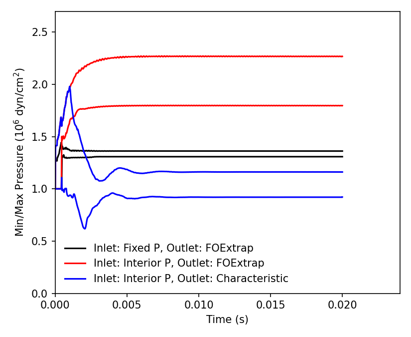
This figure shows the minimum and maximum pressures in the domain as a function of time for each boundary condition specification. The first two approaches, which ignore the transfer of information through characteristics, result in unphysical behavior. In the first, the pressure ratio across the nozzle is incorrect. In the second, the pressure ratio is correct once the system reaches a steady state, but no boundary condition fixes the pressure, so the magnitude of inlet and outlet pressure evolve to undesired values. The third set of boundary conditions leads to the desired behavior, with the outlet pressure fixed at the specified value and the inlet pressure having the appropriate relationship given the inlet Mach number and area ratio across the nozzle (Note, in this figure the maximum and minimum pressures in the domain go slightly above and below the inlet and outlet pressures due to three-dimensional effects. As shown above, the inlet and outlet pressures on the centerline match the theoretically predicted values).
Running study
mpi_ranks=36

for i_in in 0 1; do
    for i_out in 0 1; do
        dirname=run_$i_in$i_out
        echo $dirname
        mkdir $dirname
        cp example.inp $dirname/run.inp
        cd $dirname
        sed -i "s/prob.inlet_type = 0/prob.inlet_type = $i_in/g" run.inp
        sed -i "s/prob.outlet_type = 0/prob.outlet_type = $i_out/g" run.inp
        srun -n ${mpi_ranks} ../PeleC3d.gnu.MPI.ex run.inp
        cd ..
    done
done

# change path to AMReX fextract utility executable as appropriate
../../../Submodules/PelePhysics/Submodules/amrex/Tools/Plotfile/fextract.gnu.ex run_01/plt24000

# Requires: Python3 Numpy Scipy Pandas Matplotlib
python plot.py